Welcome back! In the last lesson, we performed inverse rendering to optimize camera parameters. In this lesson, we will perform one last inverse rendering experiment and optimize mesh vertex parameters.

Contents

Optimizing Mesh Vertices

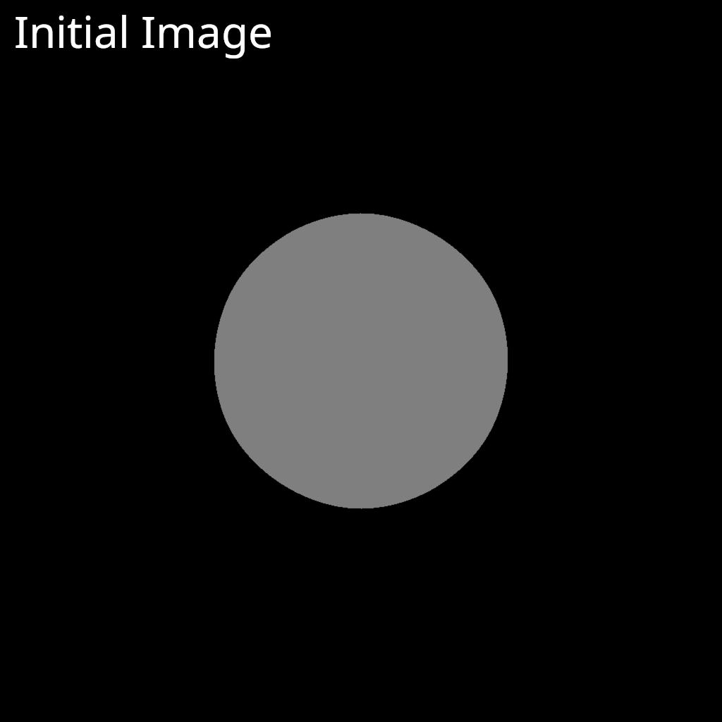
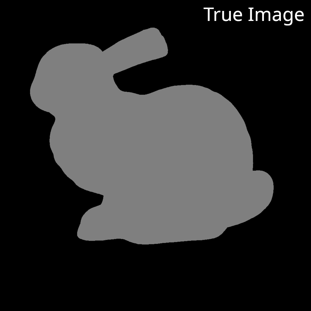
We will start by a rendering a ground truth image of a mesh. Next, we will create another pipeline with a different initial mesh. The optimization process will attempt to update the vertices of the initial mesh to match the ground truth image using gradient descent.

Here, we will use the stanford bunny mesh as the ground truth geometry, and a sphere mesh as the initial geometry.

The true and initial renderings for our mesh optimization experiment.

Let’s see what happens when we press go!

The mesh optimization process without any regularization.

Overall, this is not a bad start… but it’s not great either. The gradient computation appears to be working well because the mesh is deforming to match the shape of the bunny. The issue is that the topology of the mesh is becoming extremely messy in the process. This prevents it from converging to a decent result. A small number of triangles are becoming much larger than the others and dominating the optimization process. Can you think of anything that we could do to address this issue?

This is actually quite a difficult problem to solve in general. We need some way of informing our optimization algorithm that we want our mesh to retain some degree of regularity. As you can imagine, there are many ways of defining regularity and the best choice will usually be problem specific. One simple and general form of regualization that we will implement here is edge length regularization. This means that we will add a second loss that measures how much the triangle edge lengths of the mesh diverge from their initial lengths. The result of this will be that our optimization process will have two sources of (possibly competing) gradients. One source (the image matching loss) will pull the triangle vertices to match the reference image. The other source (the regularization loss) will pull the triangle vertices so that the edge lengths match those of the original mesh. Let’s see what happens to our optimization process when we implement this.

The mesh optimization process with edge length regularization.

Clearly, the regularization loss is working to prevent the mesh from becoming scrambled as before. Unfortunately, this also means that the mesh is unable to deform enough to closely match the target image. Let’s try another experiment where we periodically reset the reference edge lengths. This will still provide some of regularization, but should also, over time, allow the mesh to undergo the large transformations required in this example. Here is what this looks like.

The mesh optimization process with edge length regularization and periodic edge length resets.

This is starting to look a bit better now, but several issues still remain. For one, we have introduced a tradeoff in our optimization procedure. We must now compromise between minimizing our image-based rendering loss and minimizing our edge length loss that seeks to retain mesh regularity. Periodically re-setting edge lengths is a relatively hacky heuristic to alleviate this issue. Another important issue is that the addition of regularization makes the optimization procedure take considerably more time to run. Hopefully, you can now see that a differentiable rendering algorithm alone does not make the optimization of mesh geometry an easy problem to solve.

Thankfully, this is an active area of research and several innovative approaches have been proposed to improve mesh geometry optimization. One approach that we believe is particularly worth mentioning is the use of pre-conditioned gradient descent optimization as proposed in the 2021 paper “Large Steps in Inverse Rendering of Geometry” by Baptiste Nicolet, Alec Jacobson, and Wenzel Jacob. In their approach, there is an additional step that occurs before each variable update. The role of this additional step is to spread out the gradient information across the entire mesh in a smooth way, thereby enabling convergence using fewer and larger steps while retaining a regular mesh. Covering this approach in detail is slightly out of scope for this course, which aims to focus on differentiable rasterization algorithms, but would be an excellent bonus implementation challenge for anyone who wishes to expand their knowledge of geometry optimization.

Coding Challenge 11

The coding challenge for this lesson is replicate the experiments shown above and optimize some mesh vertex parameters. Again, we simply need another training loop in which we iteratively backpropagate gradients from the loss to the vertex parameters, and then use the gradients to update the parameters. We will also provide more detail on our edge length regularizer below.

Implementation

An edge length regularizer is actually quite simple. Our entire implementation can be found below. We chose to use some python language features because the availability of a hash set makes things significantly simpler. The build_connections() function will also only run once when the class is instantiated.

@ti.data_oriented
class EdgeLengthRegularizer:

    def __init__(self, mesh: TriangleMesh, weight: float = 1.0):
        self.mesh = mesh
        self.weight = ti.field(dtype=float, shape=())
        self.weight[None] = weight

        # Allocate fields
        self.loss = ti.field(dtype=float, shape=(), needs_grad=True)

        # Build data structures for vertex-vertex connections
        self.build_connections()

        # Initialize the edge lengths used as reference
        self.set_reference_edge_lengths()

    def forward(self):
        self.clear()
        self.compute_loss()

    def clear(self):
        self.loss.fill(0)

    def backward(self):
        self.loss.grad.fill(1.0)
        self.compute_loss.grad()

    @ti.kernel
    def compute_loss(self):
        for e in self.edges:
            v0 = self.mesh.vertices[self.edges[e][0]]
            v1 = self.mesh.vertices[self.edges[e][1]]
            length = tm.distance(v0, v1)
            reference_length = self.edge_lengths[e]
            self.loss[None] += self.weight[None]*(length - reference_length) ** 2

    @ti.kernel
    def set_reference_edge_lengths(self):
        for e in self.edges:
            v0 = self.mesh.vertices[self.edges[e][0]]
            v1 = self.mesh.vertices[self.edges[e][1]]
            self.edge_lengths[e] = tm.distance(v0, v1)

    def build_connections(self):
        # Using raw python here because I don't want to manually implement a hash set in Taichi 
        edges = set()
        for t in range(self.mesh.n_triangles):
            verts_ids = self.mesh.triangle_vertex_ids[t] - 1
            edges.add(frozenset([verts_ids[0], verts_ids[1]]))
            edges.add(frozenset([verts_ids[1], verts_ids[2]]))
            edges.add(frozenset([verts_ids[2], verts_ids[0]]))

        # Store the edges as a field
        n_edges = len(edges)

        self.edges = ti.Vector.field(n=2, dtype=int, shape=(n_edges))
        self.edges.from_numpy(np.array([list(e) for e in edges]))

        # Create another field to store the edge lengths
        self.edge_lengths = ti.field(dtype=float, shape=(n_edges))

Conclusion

In this lesson, we implemented our fourth inverse rendering experiment! We have now used a differentiable rasterization pipeline to implement inverse rendering for light, material, camera, and geometry parameters. In the next (and final) lesson, we will conclude the course with a discussion of what we learned, and where one could go from here to continue exploring the world of inverse rendering.