10) Optimize Camera Parameters
Welcome back! In the last two lessons, we implemented two different approaches to solve the discontinuity problem in our rasterization pipeline. We also used Jacobian images to check that both of them produced valid gradients at silhouette boundaries. In this lesson, we will do some more inverse rendering and use both approaches to optimize camera parameters. Thankfully, we have implemented all of the difficult code already. If you’ve made it this far, the course should be smooth sailing from here on out!
Contents
Optimizing Camera Parameters
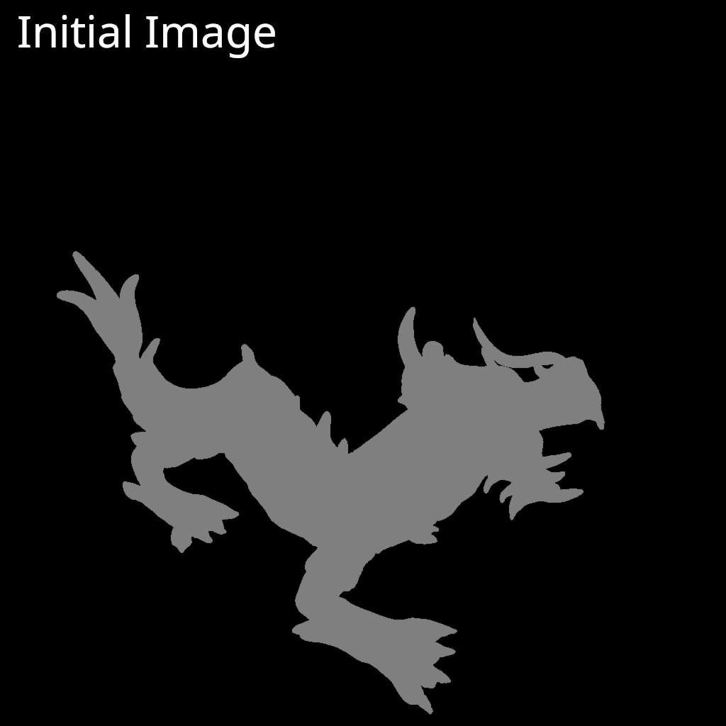
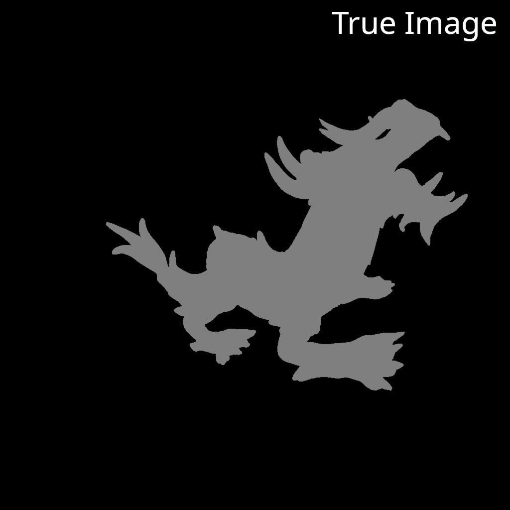
We will start by constructing a pipeline using one set of camera parameters, and rendering a ground truth image. We will use a silhouette shaded image again so that the only possible source of gradient information comes from silhouette boundaries. Next, we will perturb the camera parameters away from their ground truth values. Finally, we will see if we can recover the original camera parameters using gradient descent by comparing rendered images to the ground truth image.
Here is a figure showing true and initial images of a dragon mesh (obtained from the Stanford 3D scanning repository) rendered with silhouette shading.


RTS
Here is a video showing the process of gradient descent optimization using the RTS approach to solve the discontinuity problem We can see that the original camera parameters are recovered!
NVDR
Here is a video showing the process of gradient descent optimization using the NVDR approach to solve the discontinuity problem
Again, the original camera parameters are recovered! For this experiment, using the RTS approach with an identical learning rate leads to slightly faster convergence compared to NVDR. This could indicate that RTS produces slightly larger magnitude gradients compared to NVDR. Using a Nvidia 2070 super GPU, we also notice that the NVDR experiment trains at a slightly higher framerate (~75 fps) compared to RTS (~65 fps). This small difference may be a reflection of our implementation rather than the algorithm as we have not performed extensive optimization.
Food For Thought
Did you notice that image begins to shake in the experiments above once the rendered dragon image overlaps the true dragon image almost completely. Can you think of why that is happening? Can you think of a way to prevent it from happening so that the optimization smoothly settles on a final parameter configuration?
In the experiments above, the true and initial images of the dragon are partially overlapping. What do you think would happen to the optimization process if they did not overlap at all? Given that the optimization process is path-dependent, is it possible that the optimization process could fail to converge to an optimal solution? What sort of scenarios would lead to a local minimum or plateau in the loss landscape from which the gradient descent algorithm may not escape. Are there any techniques that you could employ to prevent the optimization process from becoming stuck?
Coding Challenge 10
The coding challenge for this post is replicate the experiments shown above and optimize some camera parameters. If you have been keeping up with the coding challenges thus far, this will be another fairly straighforward application of the Taichi AD system. We simply need another training loop in which we iteratively backpropagate gradients from the loss to the camera parameters, and then use the gradients to update the parameters. As always, you can also go look at the project codebase to see exactly how our implementation works.
Conclusion
In this lesson, we used both the RTS approach and the NVDR approach to solve the discontinuity problem and optimize camera parameters from a ground truth silhouette image. We have now validated both the RTS and NVDR approaches using Jacobian images and optimization experiments! In the next lesson, we will perform one final inverse rendering experiment and optimize the mesh vertex parameters.