9) Nvidia Diff Rast (NVDR)
Welcome back! In this lesson we will be diving into the 2020 paper Modular Primitives for High-Performance Differentiable Rendering by Laine et al. This paper describes the approach called Nvidia Diff Rast (NVDR). This is the second paper that we will review and implement in order to solve the discontinuity problem in our rasterization pipeline.
Contents
Discussion
Overview
We will begin with an overview of the NVDR approach. The core idea of NVDR is to use a distance-to-edge antialiasing (AA) operation to smooth the discontinuities that occur at silhouette boundaries. The degree of smoothing in the AA is continuously related vertex positions. Therefore, gradients at silhouette boundaries can be backpropagated by AD systems.
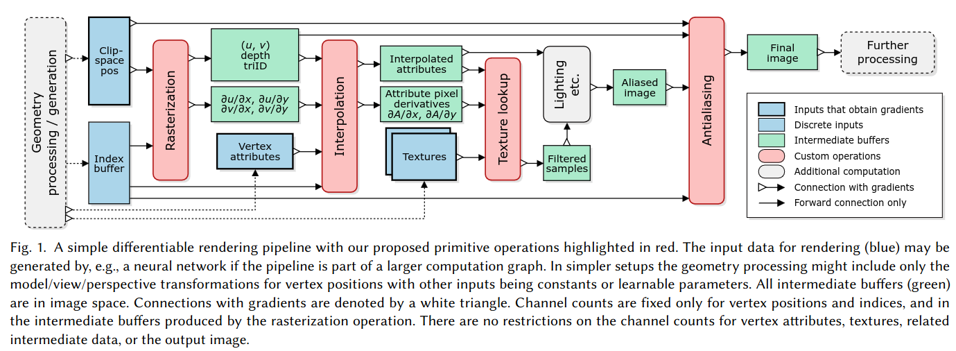
Going through the overview diagram we can see, once again, that we already have most of what we need to implement this in our codebase! We have a rasterization class that produces barycentric, depth, and triangle id buffers. We have an attribute interpolator class, and a class to perform shading. We are not going to be performing texture lookup in our codebase so we will ignore that aspect of the diagram. This means that the only thing we are missing is a the AA operation. Let’s now take a closer look at their proposed AA operation.
Distance-to-Edge Antialiasing
Aliasing is a phenomenon that can occur when signals or images are sampled at low frequencies, creating distortions or artifacts. Typically, AA techniques are applied in order to remove or mitigate the effects of aliasing. The process of rasterization involves sampling an image and can therefore produce aliasing artifacts. One common artifact seen in rasterization is that straight edges can appear jagged in an image. This occurs when pixel color is based on a single sample at the center of each pixel. Even if a triangle partially overlaps a pixel, it has no effect on the pixel color unless the triangle overlaps the pixel center. AA operations can be used to reduce the jagged appearance of edges in an image.

One simple approach to AA in rasterization is to sample the image multiple times in each pixel. The color of the pixel can then be computed as the average color of all samples. In this approach, a triangle that partially overlaps a pixel can influence the pixel color if it overlaps any of the multiple samples. This results in smoother looking (less jagged) edges, but also incurs a significant computational cost.
An alternative approach to reduce the jagged appearance of lines is called distance-to-edge AA. In this approach, an operation is performed to blend the color of pixels on either side of an edge based on the distance from the edge to each pixel. This also has the effect of reducing the jagged appearance of edges, and can be less computationally expensive than evaluating multiple samples at each pixel. The developers of NVDR had the insight that distance-to-edge AA can also be applied to solve the discontinuity problem! It smooths out the hard silhouette boundaries that are the cause of the discontinuity problem, and does so in a way that continuously relates pixel color to vertex positions.
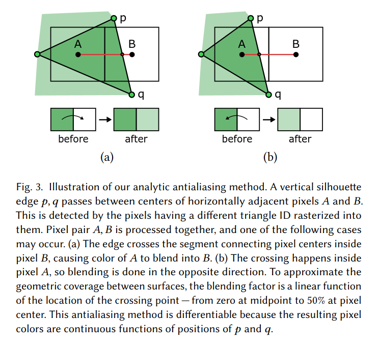
The blending operation described in the figure above is very simple to implement. It simply requires one to find the point where a silhouette triange edge passes between two pixels (A and B). If the crossing point is within pixel A, then pixel A is blended with pixel B. If the crossing point is within pixel B, then pixel B is blended with pixel A. The challenging aspect of this approach is detecting which pairs of pixels should be blended. This blending operation should only be applied at silhouette edges and not across the entire image.
Detecting Silhouette Edges
The approach to determine which pixels to blend in the NVDR AA operation proceeds as follows. First, all pairs of neighbor pixels (both vertical and horizontal) with different triangle ids in the triangle id buffer are identified as candidates for blending. Neighbor pixels with the exact same triangle id cannot be bisected by a silhouette edge because they are both within a single triangle. Next, each pair of candidate pixels is processed. The triangle id from the pixel that is closer to the camera is selected and the associated vertex coordinates are retrieved. The vertex coordinates are used to determine which of the three triangle edges intersects the line segment connecting the two pixel centers. Next, the orientation of the edge is checked. For horizontal pixel pairs, only vertical edges (with slope \(>45^\circ\)) are candidates for blending, and vice versa. Finally, a check is performed to determine if the edge is a silhouette edge.
The first step in checking if an edge is a silhouette is to find which, if any, other triangles in the mesh share the same edge. In order to find all triangles associated with an edge in an efficient way, an additional data structure (such as a hash map or lookup table) must be constructed. If the edge is not shared by any other triangle, it is a silhouette edge and blending is performed. If the edge is shared by another triangle, an additional test is performed to see if both triangles lie on the same side of the edge in screen space. If they do, the edge is a silhouette edge and blending is performed.
Limitations
This approach has a couple of limitations that are worth mentioning. The first is that edge to triangle lookups require an additional data structure to be performed efficiently. The second is that this approach may not blend all pixels pairs that are bisected by silhouette edges. This is especially common when using images with low resolution and meshes with large numbers of very small triangles. Here is a quick diagram to illustrate how this can happen.
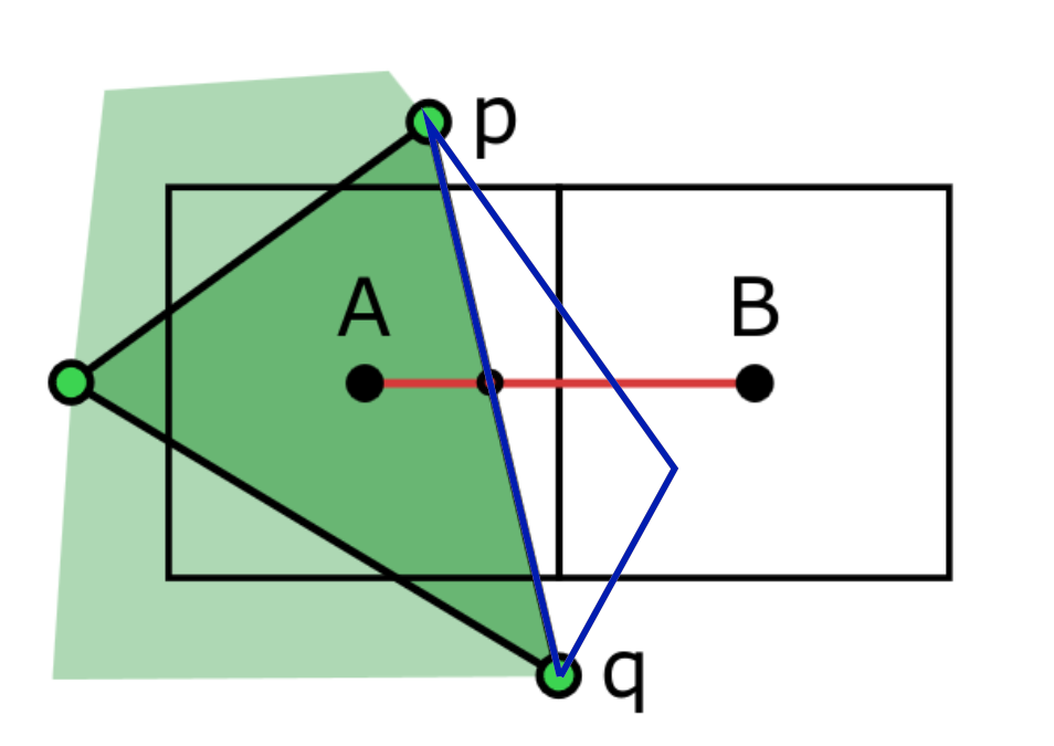
In this example we could imagine that the pixel pair \((A,B)\) was processed up until the point of checking if edge \((p,q)\) of the green triangle was a silhouette edge. The edge triangle lookup would be performed, and it would be found that edge \((p,q)\) is shared with another triangle (blue) on the oposite side of the edge. Therefore, \((p,q)\) is not a silhouette edge and pixel pair \((A,B)\) would not be blended even though it is bisected by a genuine silhouette edge!
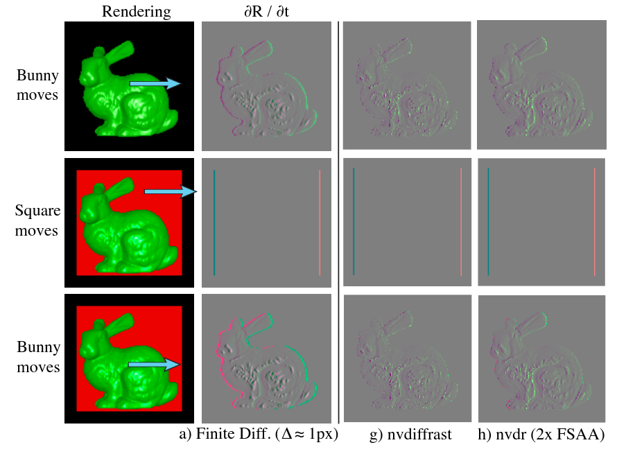
This limitation is discussed in the NVDR paper and was also adressed in the RTS publication by Cole et al. Here you can see a figure from the RTS publication showing how the NVDR gradients at the boundary of the bunny image are quite poor due to many missed silhouette pixel pairs. They also double the resolution of the image (2x FSAA) to address this problem with only partial success.
Improved Silhouette Detection
Before we move onto the implementation and results, can you think of any ways that we could improve this silhouette detection algorithm? Ideally, we would like to avoid missing sillhouette pixel pairs because we know that it can impact the quality of the gradients. Additionally, it would be nice if we didn’t need to build a data structure for edge to triangle lookups. Actually… didn’t we just implement a form of silhouette detection for the RTS approach?
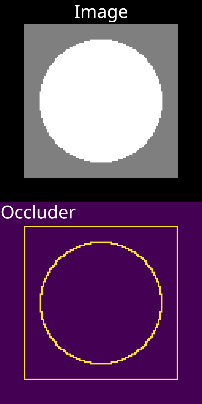
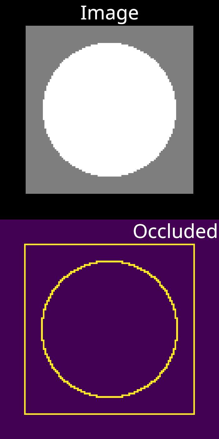
In our RTS implementation, we used multi-layer rasterization buffers to identify which pixels are occluders and which are occluded. For this application, we also need to capture silhouette boundaries against the image background, but that is a fairly simple adjustment. Here are some buffers that we can produce using that approach. Once again, we will use the example scene of a spherical mesh in front of a plane.
Let’s consider a different version of the NVDR AA operation that has access to these buffers. Any pair of neighbor pixels, where one is an occluder and the other is occluded, will be treated as if they are bisected by a silhouette edge. We will ignore rare cases where pixels both occlude and are occluded (these pixels will not be blended). The triangle id of the occluder pixel will be used to access a triangle and the corresponding vertex coordinates. The triangle edge that intersects the line segment between pixels will found and used to perform blending, if it is oriented properly (using the same criterion as the original algorithm).
Does this sound like an improved method to you? It does not require any edge to triangle lookups and therefore does not require a hash map or lookup table. It will also not miss any pixels pairs that bisect a silhouette edge. The downsides are that it requires a two layer rasterization buffer whereas the original approach does not. Additionally, the blending operation will not necessarily be performed using distance to the silhouette edge, but rather the distance to the edge of the triangle whose id is in the occluder pixel. However, this is still a better outcome than no blending at all.
Whether or not this can be considered an improved algorithm, it will simplify our implementation of the NVDR AA operation considerably by letting us re-using code that we have already written. Therefore, this is the approach that we take in our codebase.
Results
Let’s now take a look at some results. We will continue to use the example of a sphere mesh in front of a plane mesh. To begin, let’s see how the output of the antialiasing operation compares to the the splatting operation from the RTS approach.
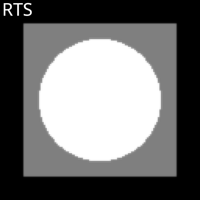
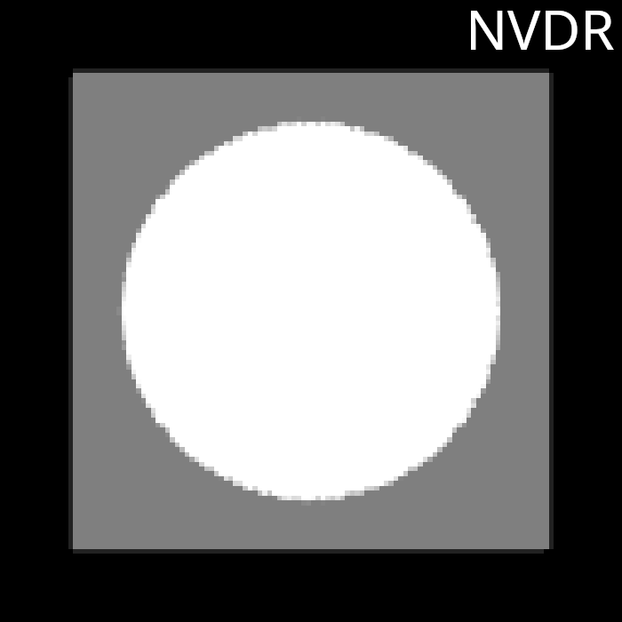
Overall, the result is quite similar in that the silhouette boundaries are blurred. The NVDR blurring appears to be bit less uniform compared to RTS. Althought it is not visible with this example, we should also remember that NVDR only blurs silhouette boundaries while RTS blurs the entire image.
Jacobian Images
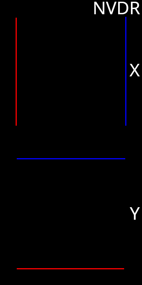
We should also check our gradients using Jacobian images and compare them to the RTS approach. First let’s visualize Jacobian images with respect to x and y translation of the sphere mesh.
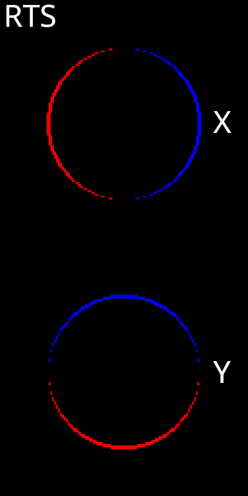
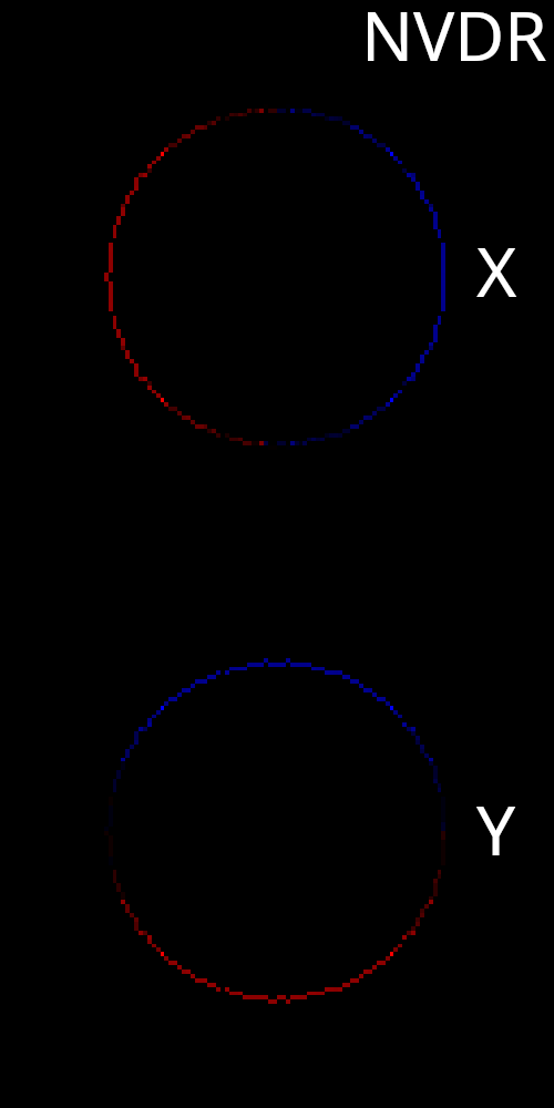
While there are some differences between the two, it is clear that NVDR is also correctly capturing the effect that translating the sphere will have on the resulting image. Again, the NVDR gradients appear to be slightly less uniform compared to RTS. Additionally, the boundary gradients have slightly less spatial thickness compared to RTS. It is possible that this could have some small effect on optimization experiments. Now we move on to visualize Jacobian images with respect to x and y translation of the plane mesh.
Again, NVDR is correctly capturing the effect that translating the plane will have on the resulting image. Unlike RTS, we don’t need to make any adjustments to the approach to correct spurious gradients for this scenario.
Coding Challenge 9
The coding challenge for this lesson is to implement the NVDR approach and generate some Jacobian images to confirm that the gradients are working properly. Some additional discussion about our implementation can be found below. You can also go look at the project codebase to see exactly how our implementation works.
Implementation
There is only one additional class that we need to implement the NVDR approach into our codebase. That is, of course, a class to perform antialiasing. This class needs access to a shaded image buffer, the mesh vertices in clip coordinates, and the vertex ids of each triangle in the mesh. Additionally, the class has an occlusion estimator as a member, which accesses a depth buffer and a triangle id buffer.
Our implementation uses two kernels. The first kernel parallelizes over each occluder pixel, and computes blending factors for all four neighbor pixels (up, down, left, right). The second kernel parallelizes over all pixels and applies a blending operation when required.
It’s also important to take note the gradient flow for this operation. Gradients flow from the output buffer back to the shade buffer. Additionally, gradients flow back to the clip space vertex buffer which resides in our rasterizer. These gradients are acumulated with other gradients from the barycentric buffer when backward is called on the rasterizer. RTS treated rasterization as a non-differentiable sampling process, and therefore we do propagate gradients through the rasterizer. NVDR treats rasterization as differentiable, and requires that gradients also propagate through the rasterizer.
@ti.data_oriented
class Antialiaser:

    def __init__(
        self,
        shade_buffer: ti.Vector.field,
        depth_buffer: ti.field,
        triangle_id_buffer: ti.field,
        clip_vertices: ti.Vector.field,
        triangle_vertex_ids: ti.Vector.field,
    ):
        self.shade_buffer = shade_buffer
        self.triangle_id_buffer = triangle_id_buffer
        self.clip_vertices = clip_vertices
        self.triangle_vertex_ids = triangle_vertex_ids

        self.x_resolution = shade_buffer.shape[0]
        self.y_resolution = shade_buffer.shape[1]

        self.occlusion_estimator = OcclusionEstimator(
            depth_buffer=depth_buffer,
            triangle_id_buffer=triangle_id_buffer,
            background_occlusion=True,
        )

        # The blend factor field stores how much each occluder pixel is blended with neighbor pixels
        # The 4 values per pixel correspond to neighbors in the order of [up, down, left, right]
        self.blend_factor_buffer = ti.field(
            dtype=float,
            shape=(self.x_resolution, self.y_resolution, 4),
            needs_grad=True,
        )

        self.output_buffer = ti.Vector.field(
            n=3,
            dtype=float,
            shape=(self.x_resolution, self.y_resolution),
            needs_grad=True,
        )

    def forward(self):
        self.clear()
        self.occlusion_estimator.forward()
        self.compute_blend_factors()
        self.blend()

    def backward(self):
        self.blend.grad()
        self.compute_blend_factors.grad()

    def clear(self):
        self.output_buffer.fill(0)
        self.blend_factor_buffer.fill(0)
        self.output_buffer.grad.fill(0)
        self.blend_factor_buffer.grad.fill(0)

    @ti.kernel
    def compute_blend_factors(self):
        for x, y in ti.ndrange(self.x_resolution, self.y_resolution):

            pix_is_occluder = self.occlusion_estimator.is_occluder_buffer[x, y]
            if pix_is_occluder:

                # Get vertices in screen space
                triangle_id = self.triangle_id_buffer[x, y, 0]
                vert_ids = self.triangle_vertex_ids[triangle_id - 1] - 1

                v0_clip = self.clip_vertices[vert_ids[0]]
                v1_clip = self.clip_vertices[vert_ids[1]]
                v2_clip = self.clip_vertices[vert_ids[2]]

                v0_screen = ndc_to_screen(
                    v0_clip.xy / v0_clip.w, self.x_resolution, self.y_resolution
                )
                v1_screen = ndc_to_screen(
                    v1_clip.xy / v1_clip.w, self.x_resolution, self.y_resolution
                )
                v2_screen = ndc_to_screen(
                    v2_clip.xy / v2_clip.w, self.x_resolution, self.y_resolution
                )

                # Compute and set the blend factors for each neighbor
                for i in ti.static(range(4)):
                    self.compute_blend_factor(
                        v0_screen, v1_screen, v2_screen, ivec2([x, y]), i
                    )

    @ti.kernel
    def blend(self):
        for x, y in self.output_buffer:
            pix_is_occluder = self.occlusion_estimator.is_occluder_buffer[x, y]
            pix_is_occluded = self.occlusion_estimator.is_occluded_buffer[x, y]

            # If pix is neither occluded nor occluder, pass it through untouched
            if (not pix_is_occluded) and (not pix_is_occluder):
                self.output_buffer[x, y] = self.shade_buffer[x, y, 0]

            else:
                # Grab the blend factors
                up_blend = self.blend_factor_buffer[x, y, 0]
                down_blend = self.blend_factor_buffer[x, y, 1]
                left_blend = self.blend_factor_buffer[x, y, 2]
                right_blend = self.blend_factor_buffer[x, y, 3]

                # Normalize in rare case blend factors sum to > 1
                blend_sum = up_blend + down_blend + left_blend + right_blend
                blend_normalization = 1.0 if blend_sum < 1 else blend_sum
                pixel_blend = 0.0 if blend_sum > 1 else 1.0 - blend_sum

                # Blend
                pixel_color = self.shade_buffer[x, y, 0]
                up_color = self.shade_buffer[x, y + 1, 0]
                down_color = self.shade_buffer[x, y - 1, 0]
                left_color = self.shade_buffer[x - 1, y, 0]
                right_color = self.shade_buffer[x + 1, y, 0]

                output_color = (
                    pixel_color * pixel_blend
                    + up_color * up_blend / blend_normalization
                    + down_color * down_blend / blend_normalization
                    + left_color * left_blend / blend_normalization
                    + right_color * right_blend / blend_normalization
                )

                self.output_buffer[x, y] = output_color
Conclusion
In this lesson, we covered the NVDR approach to solving the discontinuity problem. We saw how distance-to-edge antialiasing can be used to turn hard discontinuous boundaries into soft continuous boundaries. We have now reviewed and implemented two state of the art approaches for solving the discontinuity problem in a rasterization pipeline!