4) Shading
Welcome back! In the last lesson, we implemented a triangle rasterizer that takes a camera and a triangle mesh and produces three image buffers (triangle id, barycentric coordinates, and depth). In this lesson we will be continuing along the forward direction of our rasterization pipeline and, at last, producing shaded images of some triangle meshes. This means that we are nearing the end of our journey through the forward pass and will soon begin looking at gradients!
Contents
Discussion
Shading is the process of computing the apparent color of objects in a 3D scene. The color of an object is dependent on several things. For one, the light that is incident upon the object will influence it’s appearance. Incident light can differ in terms of intensity, wavelength, polarization, and direction. In most scenes there will be multiple sources of light. Another factor that influences the appearance of an object is the geometry of the object. Light will interact with objects differently depending on the position and orientation of an object relative to the incident light. Furthermore, objects will appear different depending on properties of the camera. Finally, the material properties of an object will have an effect on it’s appearance. Light interactions will differ if the object is black/white, or shiny/rough, or opaque/translucent. Many different approaches have been developed to model each of these different properties and how they affect light transport. As you can probably imagine, these models can become extremely complicated.
In this project we will make many simplifying assumptions about the scene that is being rendered and the process of light transport. Just as we discussed when introducing rasterization, this means that we will not be able to simulate every aspect of real-world light transport. This is not a bad thing! Trying to model all aspects of light transport at once is not at all a good way to begin. Statistician George Pox once said “All models are wrong, but some are useful”. Our model will be wrong in many respects, but it will also be useful. We must simply be alert to how it is wrong, and how it is useful.
In this project, we will ignore light polarization (and the quantum nature of light for that matter) and represent light color using a simple RGB decomposition as opposed to a continuous wavelength representation. We will use a very simple model for light emmission (directional lights), and a very simple model for material properties (albedo only). We will represent 3D objects using opaque, triangular surface meshes. We will ignore indirect illumination of any kind, and we will even ignore shadows. As a result of these simplifying assumptions, our shading algorithm will be simple to implement, computationally efficient and will still capture many interesting phenomena. By the end of the project, we will be able to learn scene parameters for light, geometry, camera, and material properties. We will also have an excellent perspective from which to identify the shortcomings of our model, and think of ways in which one could develop more sophisticated models to capture more, and more interesting, optical phenomena.
Blinn-Phong Shading
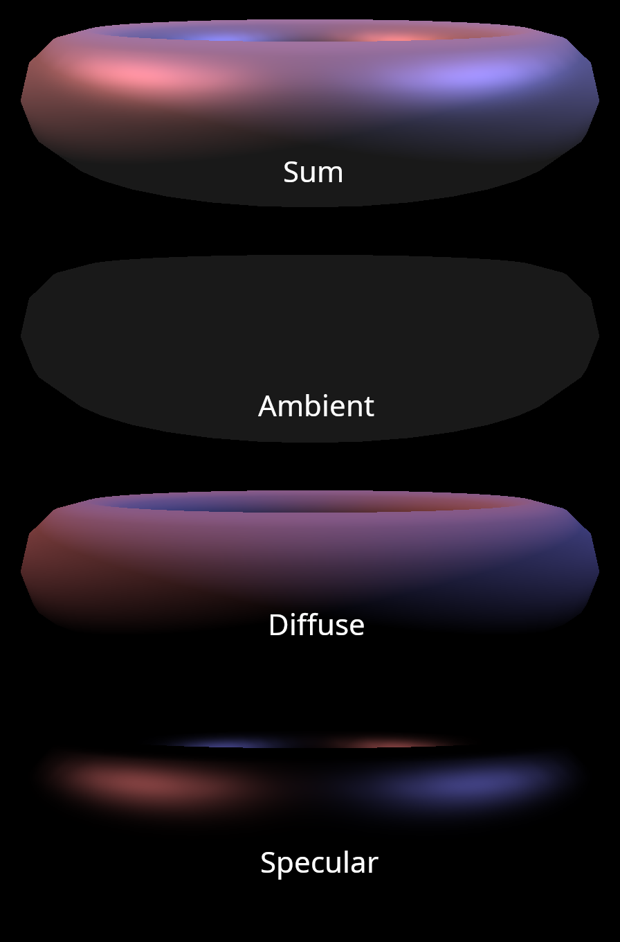
Thanks to our hard work in the last lesson, we now have a rasterization approach that determines triangle coverage for an image. This information is captured in image buffers that store the id, barycentric coordinates, and depth of triangles at each pixel. To compute the final pixel color for our image, we will use the Blinn-Phong shading algorithm. This is a simple and classic approach that has been used in many graphics pipelines. The Blinn-Phong shading model is the sum of three individual components, ambient, diffuse and specular. The ambient component represents light that is emmitted from a surface regardless of incident light. The best way to think about the ambient component is as a fudge factor that very loosely approximates the effect of indirect illumination. The diffuse component approximates the effect of direct light that is reflected by a rough or matte surface. The specular component approximates the effect of direct light that is reflected by a shiny surface.
Let’s look at a simple example to get a better sense of what this looks like. Here is a rendering of a white torus mesh that is illuminated by two directional lights. One of the lights has a red tint, and the other has a blue tint. We can visualize each component individually, and then sum them up to produce a final rendering of the mesh.
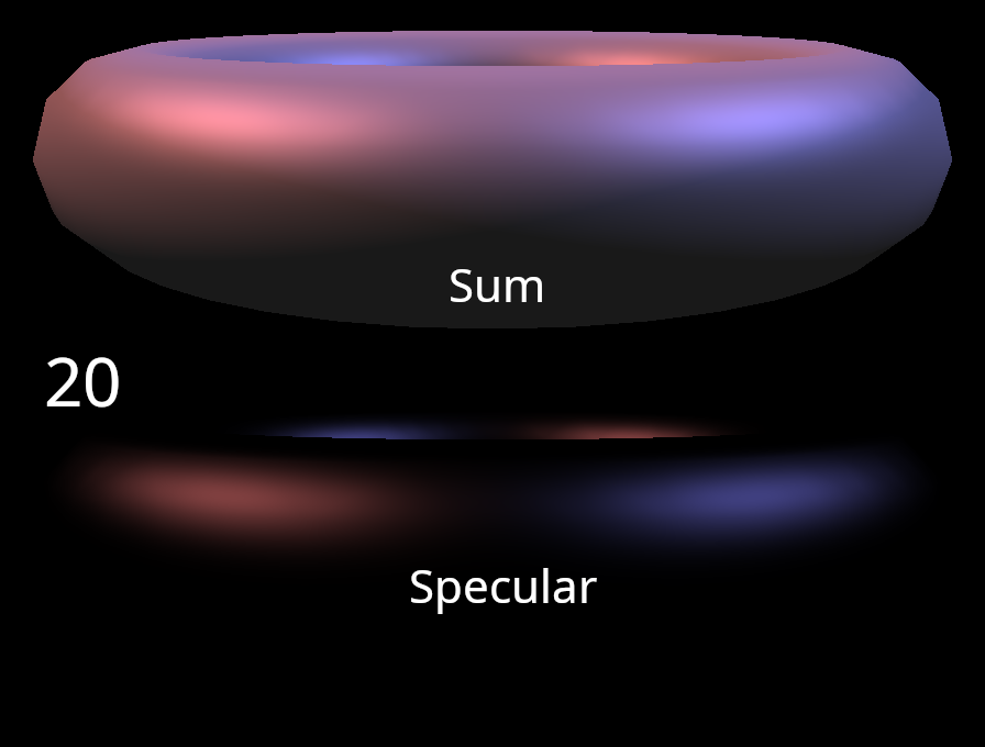
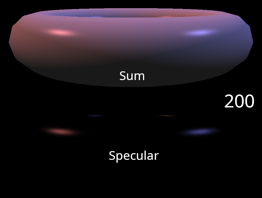
The Blinn-Phong shading approach also includes a specular exponent parameter to control the width of the specular lobe. A larger exponent results in a narrower specular lobe which gives the impression of a shinier object. You can see the difference in the figure below.
Let’s now take a look at the math behind each component a bit more closely. The ambient component is the simplest as it is intependent of any incident light. The ambient component is simply equal to the albedo of the surface (\(\alpha\)) multiplied by some scalar constant controlling it’s overall magnitude (\(C_{a}\)).
\begin{equation} I_{a} = C_{a} \; \alpha \end{equation}The other two components require additional information about the geometry and light incident upon the surface at each point. This information is captured by several vectors illustrated in the image below.
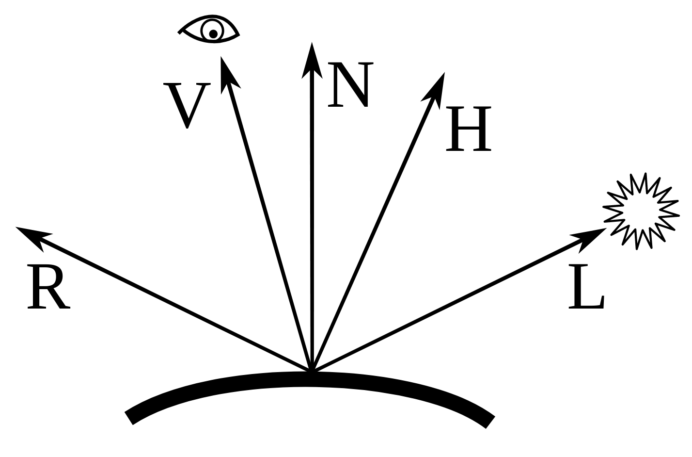
The diffuse component is equal to a constant \(C_{d}\), multiplied by the albedo of the surface, multiplied by the incident light \(I_i\) attenuated by the cosine of the angle of incidence. The attenuation term can be computed by taking the inner product of the light unit vector (denoted L in the image above) with the surface normal unit vector (denoted N in the image above). Thus, the cosine attenuation term falls to zero when the incident light direction is perpendicular to the surface normal.
\begin{equation} I_d = C_d \; \alpha \; I_{i} \; \text{max}(0, \hat{n} \cdot \hat{l} ) \end{equation}Finally, the specular term is equal to a constant (\(C_s\)) multiplied by the intensity of the incident light attenuated by an exponential term. The exponential attenuation term is equal to the inner product of the normal vector with the halfway vector (denoted H in the image above) raised to the power of the specular exponent parameter (\(\beta\)). The halfway vector is a unit vector that is halfway between the light vector and the view vector (denoted V in the image above). Thus, the specular term is maximized when the view vector is equal to the light vector reflected across the axis defined by the normal vector (i.e. the reflection vector denoted R in the imag above).
\begin{equation} I_s = C_s \; I_{i} \; \text{max}(0, \hat{h} \cdot \hat{l} )^{\beta} \end{equation}For more discussion on the Blinn-Phong approach, here are several sources that cover the apprach in great detail (1, 2, 3).
G-Buffers
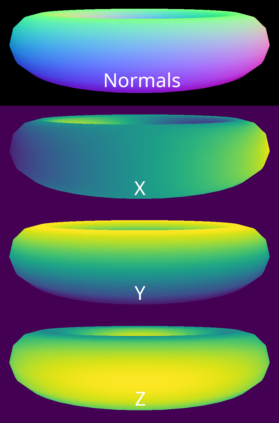
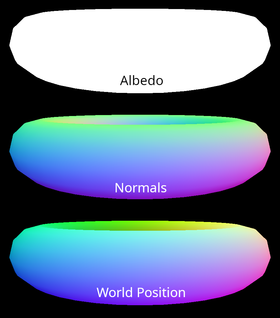
In order to produce some nice shaded images, we need additional information beyond what is provided in the output buffers from rasterization. To make this information available to a shading kernel, we create a set of G-buffers. Three G-buffers are required for our simple shading approach: albedo, normals, and world position. If we visualize the individual channels of a normal buffer, it is clear that each pixel encodes the surface normal vector for the visible point on the mesh.
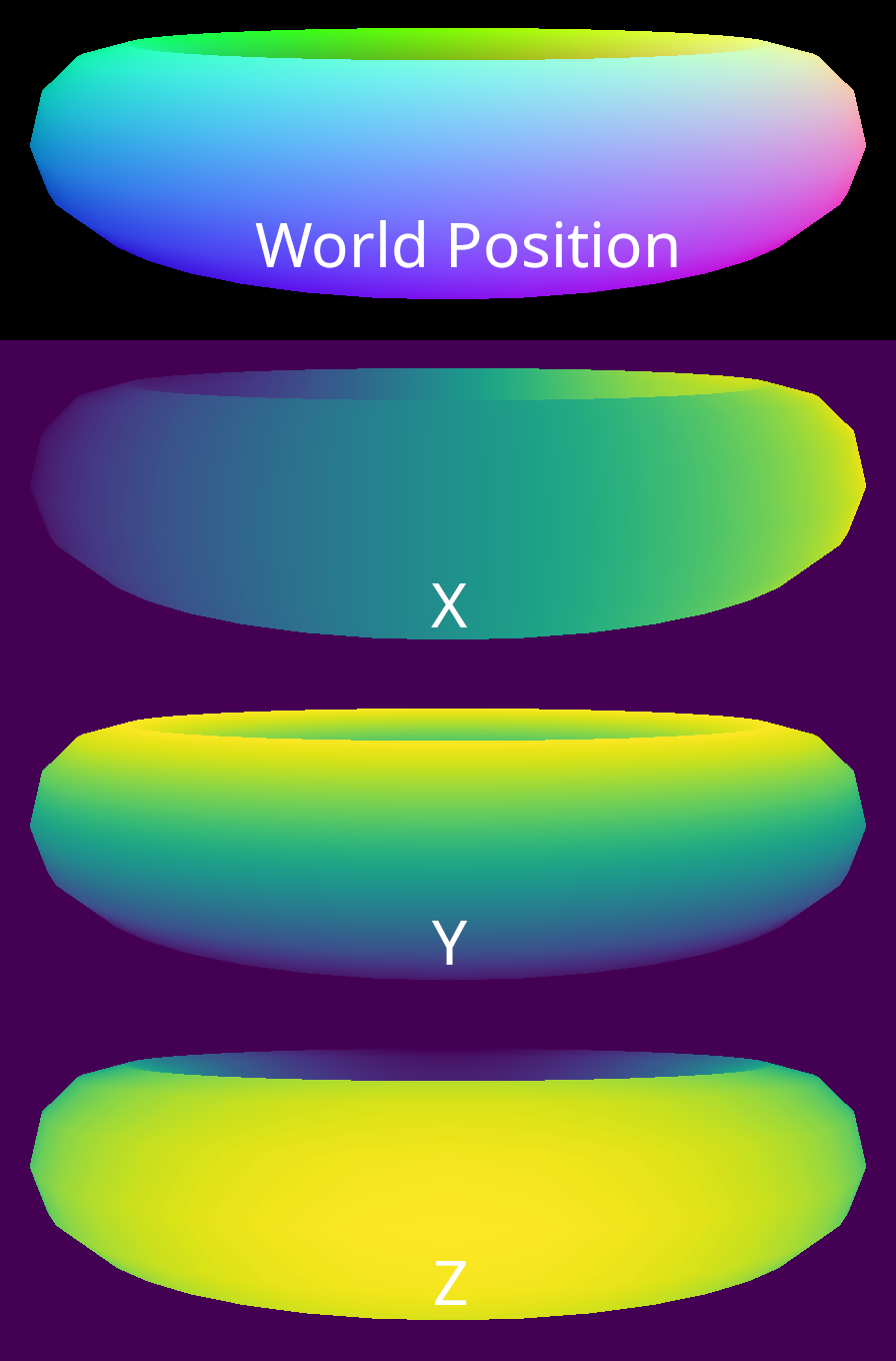
We can also do the same thing for a world position buffer. Here, each pixel encodes the position of the surface in world space for the visible point on the mesh.
The albedo buffer contains an RGB color at each pixel for the visible point on the mesh. In this example, we are using a pure white albedo for the entire mesh. Combined with information about the direction, color and intensity of the lights, these 3 buffers provide all of the information required to compute the shaded color of each pixel in the image.
Directional Lights
The final element that we require for Blinn-Phong shading is a lighting model. We are going to use directional lights, which are one of the simplest possible approaches for modelling illumination. Directional lights emit light in a specific direction such that the rays are all parallel, as if from a source that is infinitely far away. Therefore, each light must have parameters for the light direction, as well as parameters for the light color and intensity. We can combine light color and intensity into a single RGB vector.
Interactive Renderer
Similar to our rasterization demo, we set up an interactive rendering demo to explore a 3D scene. In this demo, we are visualizing the final Blinn-Phong shading result instead of the intermediate rasterization buffers. Here is a short clip of us zooming around everone’s favorite bunny (obtained from the Stanford 3D scanning repository). The lighting looks fairly good on the front of the bunny, but once we get around to the backside, the limitations of our shading approach become more obvious. For one, the ambient component is completely uniform and doesn’t allow us to discern the object geomety (unlike indirect illumination in the real world). The lack of shadows also becomes somewhat uncanny as light appears to pass through one part of the bunny to then reflect off some other part.
Nevertheless, we now have a full forward rendering pipeline implemented from scratch!
Coding Challenge 4
The coding challenge for this week is to implement Blinn-Phong shading. As always, we will provide some additional discussion about our implementation below. You can also go look at the project codebase to see exactly how our implementation works.
Implementation
Let’s begin with the G-Buffers. The world position buffer can be created by interpolating the vertex coordinates (in world space) using the barycentric coordinates in the buffer produced by the rasterizer. Likewise, the normal buffer can be created by interpolating vertex normals (in world space). Additionally, the albedo buffer can be created by interpolating per-vertex albedo values. It seems clear that we will need a class to interpolate vertex attributes.
Attribute Interpolation
A triangle attribute interpolator needs access to a vertex attribute field to be interpolated.
Furthermore, it needs access to some mesh information (triangle vertex ids), and some rasterizer outputs (triangle id and barycentric buffers) to perform the interpolation.
The output will be a buffer with the number of channels matching the dimension of the interpolated attributes.
This class can be used to interpolate world position, normals, albedo, and any other per-vertex attribute of interest.
If we want to use UV mapping in the future, we can also interpolate UV coordinates and use them to perform a lookup against an attribute image.
We will also add a boolean flag that allows us to specify that some attributes (like normals) should be unit vectors and must be normalized after interpolation.
Here is a skeleton of the attribute interpolator class.
The interpolate kernel is parallelized over every pixel in the image to maximize GPU utilization.
For each pixel, we must grab the triangle_id, look up the vertices associated with that triangle, grab the attributes associated with those vertices, and interpolate the attributes using the barycentric coordinates.
@ti.data_oriented
class TriangleAttributeInterpolator:

    def __init__(
        self,
        vertex_attributes: ti.Vector.field,
        triangle_vertex_ids: ti.Vector.field,
        triangle_id_buffer: ti.Vector.field,
        barycentric_buffer: ti.Vector.field,
        normalize: bool = False,
    ):

        self.vertex_attributes = vertex_attributes
        self.triangle_vertex_ids = triangle_vertex_ids
        self.triangle_id_buffer = triangle_id_buffer
        self.barycentric_buffer = barycentric_buffer
        self.normalize = normalize

        self.attribute_buffer = ti.Vector.field(
            n=vertex_attributes.n,
            dtype=float,
            shape=triangle_id_buffer.shape,
            needs_grad=True,
        )

    def forward(self):
        self.clear()
        self.interpolate()

    def backward(self):
        self.interpolate.grad()

    def clear(self):
        self.attribute_buffer.fill(0)
        self.attribute_buffer.grad.fill(0)

    @ti.kernel
    def interpolate(self):
        for x, y, l in self.attribute_buffer:
            pass # Your code here
Normals Estimation
We’re off to a good start, but we aren’t quite ready to write a shader class. We have a class that can interpolate normals, but we don’t yet have a way to compute normals in the first place. Computing normals for triangle faces is fairly easy, but using face normals in a shading algorithm produces images where the mesh polygons are clearly visible. We are dealing with smooth surfaces in our examples, and we would like the normals to change smoothly across our mesh to produce more realistic images. This is often called smooth shading or Phong shading. Therefore, we are going to compute normals for our mesh vertices and then interpolate them across the faces. The vertex normals will be the average of the face normals across all faces connected to a vertex, weighted by the angle of the triangle at that vertex. A way to perform this computation efficiently in Taichi is to use two kernels. The first kernel parallelizes over all triangles, computes each triangle normal vector and it’s angles, and then accumulates the normals into an intermediate buffer. The second kernel parallelizes over all vertices and simply normalizes the accumlation buffer to get the vertex normals. In this approach, we avoid duplicating computation and retain a high degree of parallelism, at the cost of maintaining an intermediate buffer. Here’s a skeleton class for estimating mesh normals.
@ti.data_oriented
class NormalsEstimator:

    def __init__(
        self,
        mesh: TriangleMesh,
    ):

        self.mesh = mesh
        self.accumulation_field = ti.Vector.field(
            n=3, dtype=float, shape=(mesh.n_vertices), needs_grad=True
        )
        self.normals = ti.Vector.field(
            n=3, dtype=float, shape=(mesh.n_vertices), needs_grad=True
        )

    def forward(self):
        self.clear()
        self.accumulate_normals()
        self.normalize()

    def clear(self):
        self.accumulation_field.fill(0)
        self.normals.fill(0)
        self.accumulation_field.grad.fill(0)
        self.normals.grad.fill(0)

    def backward(self):
        self.normalize.grad()
        self.accumulate_normals.grad()

    @ti.kernel
    def accumulate_normals(self):
        for i in range(self.mesh.n_triangles):
            pass # Your code here

    @ti.kernel
    def normalize(self):
        for i in range(self.mesh.n_vertices):
            self.normals[i] = tm.normalize(self.accumulation_field[i])
Directional Light Array
We now have the classes we need to create our G-buffers, but we still need some sort of lighting model before we can write the shader. For a directional light model, this is dead simple. Here is a Taichi class that stores an array of directional lights.
@ti.data_oriented
class DirectionalLightArray:

    def __init__(
        self,
        n_lights: int = 1,
    ):

        self.light_directions = ti.Vector.field(
            n=3, dtype=float, shape=(n_lights), needs_grad=True
        )
        self.light_colors = ti.Vector.field(
            n=3, dtype=float, shape=(n_lights), needs_grad=True
        )
Blinn-Phong Shader
Finally, we can move onto writing a Blinn-Phong shader. The shader class accesses all of the buffers described above and also has a few additional parameters. The shader processes each pixel in parallel and outputs a final shaded image buffer.
By accessing the G-buffers, the shader knows the surface position in world space, the surface normal, and the surface albedo. By accessing the light parameters, the shader also knows the light direction, color and intensity. The shader class itself contains weight parameters for the diffferent components (ambient, specular, and diffuse) as well as the shine coefficient that controls the width of the specular lobe. This is all the information required to determine the surface color using the Blinn-Phong approach.
@ti.data_oriented
class BlinnPhongShader:

    def __init__(
        self,
        camera: Camera,
        directional_light_array: DirectionalLightArray,
        triangle_id_buffer: ti.field,
        world_position_buffer: ti.Vector.field,
        normals_buffer: ti.Vector.field,
        albedo_buffer: ti.Vector.field,
        ambient_constant: float = 0.1,
        specular_constant: float = 0.1,
        diffuse_constant: float = 0.1,
        shine_coefficient: float = 10,
    ):

        self.camera = camera
        self.light_array = directional_light_array

        self.triangle_id_buffer = triangle_id_buffer
        self.world_position_buffer = world_position_buffer
        self.normals_buffer = normals_buffer
        self.albedo_buffer = albedo_buffer

        self.ambient_constant = ti.field(float, shape=())
        self.specular_constant = ti.field(float, shape=())
        self.diffuse_constant = ti.field(float, shape=())
        self.shine_coefficient = ti.field(float, shape=())

        self.ambient_constant[None] = ambient_constant
        self.specular_constant[None] = specular_constant
        self.diffuse_constant[None] = diffuse_constant
        self.shine_coefficient[None] = shine_coefficient

        self.output_buffer = ti.Vector.field(
            n=3, dtype=float, shape=albedo_buffer.shape, needs_grad=True
        )

    def forward(self):
        self.clear()
        self.shade()

    def clear(self):
        self.output_buffer.fill(0)
        self.output_buffer.grad.fill(0)

    def backward(self):
        self.shade.grad()

    @ti.kernel
    def shade(self):
        for x, y, l in self.output_buffer:
            pass # Your code here
Pipeline
We now have quite a few different rendering components, so it is helpful to create another class to keep things organized.
We create a pipeline class to hold all of the rendering components.
The pipeline also has a forward method which calls forward on all of the components in the appropriate order.
import tinydiffrast as tdr

@ti.data_oriented
class Pipeline:

    def __init__(self, resolution=(1024, 1024), mesh_type="dragon"):

        self.mesh = tdr.TriangleMesh.get_example_mesh(mesh_type)
        self.camera = tdr.PerspectiveCamera()

        self.rasterizer = tdr.TriangleRasterizer(resolution, self.camera, self.mesh, subpixel_bits=4)
        self.world_position_interpolator = tdr.TriangleAttributeInterpolator(
            vertex_attributes=self.mesh.vertices,
            triangle_vertex_ids=self.mesh.triangle_vertex_ids,
            triangle_id_buffer=self.rasterizer.triangle_id_buffer,
            barycentric_buffer=self.rasterizer.barycentric_buffer)

        self.normals_estimator = tdr.NormalsEstimator(mesh=self.mesh)
        self.normals_interpolator = tdr.TriangleAttributeInterpolator(
            vertex_attributes=self.normals_estimator.normals,
            triangle_vertex_ids=self.mesh.triangle_vertex_ids,
            triangle_id_buffer=self.rasterizer.triangle_id_buffer,
            barycentric_buffer=self.rasterizer.barycentric_buffer)

        self.vertex_albedos = ti.Vector.field(n=3, dtype=float, shape=(self.mesh.n_vertices), needs_grad=True)
        self.vertex_albedos.fill(1)
        self.albedo_interpolator = tdr.TriangleAttributeInterpolator(
            vertex_attributes=self.vertex_albedos,
            triangle_vertex_ids=self.mesh.triangle_vertex_ids,
            triangle_id_buffer=self.rasterizer.triangle_id_buffer,
            barycentric_buffer=self.rasterizer.barycentric_buffer,)

        self.light_array = tdr.DirectionalLightArray(n_lights=3)
        self.light_array.set_light_color(0, tm.vec3([1,1,1]))
        self.light_array.set_light_direction(0, tm.vec3([0,0,-1]))
        self.light_array.set_light_color(1, tm.vec3([0,1,1]))
        self.light_array.set_light_direction(1, tm.vec3([0,-1,-1]))
        self.light_array.set_light_color(2, tm.vec3([1,0,1]))
        self.light_array.set_light_direction(2, tm.vec3([-1,0,-1]))

        self.phong_shader = tdr.BlinnPhongShader(
            camera=self.camera,
            directional_light_array=self.light_array,
            triangle_id_buffer=self.rasterizer.triangle_id_buffer,
            world_position_buffer=self.world_position_interpolator.attribute_buffer,
            normals_buffer=self.normals_interpolator.attribute_buffer,
            albedo_buffer=self.albedo_interpolator.attribute_buffer,
            ambient_constant=0.1,
            specular_constant=0.2,
            diffuse_constant=0.3,
            shine_coefficient=30)

    def forward(self):
        self.camera.forward()
        self.rasterizer.forward()
        self.world_position_interpolator.forward()
        self.normals_estimator.forward()
        self.normals_interpolator.forward()
        self.albedo_interpolator.forward()
        self.phong_shader.forward()
Conclusion
In this lesson, we finished the forward pass for our renderer! We implemented some classes to create G-buffers, a simple lighting approach, and a Blinn-Phong shader. We are now ready to start discussing and implementing inverse rendering.