8) Rasterize Then Splat (RTS)
Welcome back! In this lesson we will be doing a deep dive into the 2021 paper Differentiable Surface Rendering via Non-Differentiable Sampling by Cole et al. This paper describes the approach that is colloquially called rasterize then splat (RTS). This is the first of two papers that we will review and implement in order to solve the discontinuity problem in our rasterization pipeline.
Contents
Discussion
Overview
Let’s begin with an overview of the RTS approach. The central idea of RTS is that we can take an image that has been point sampled at pixels and turn each pixel/sample into a small Gaussian “splat”. Each splat has soft boundaries and pixel values in the output image are continuously related to the splat positions.
An interesting feature of this approach is that the gradients do not flow through the rasterization operation. Rasterization is treated as a non-differentiable sampling process. The gradients instead flow through a special splat position buffer. This buffer contains the screen space coordinates of each pixel, which also define the center of each splat in screen coordinates. In other words, pixel \((x,y)\) in the splat position buffer will have a value of \((x,y)\). Here you can see a flow diagram of the approach where we have highlighted the differentiable path in green, and the non-differentiable path in red.
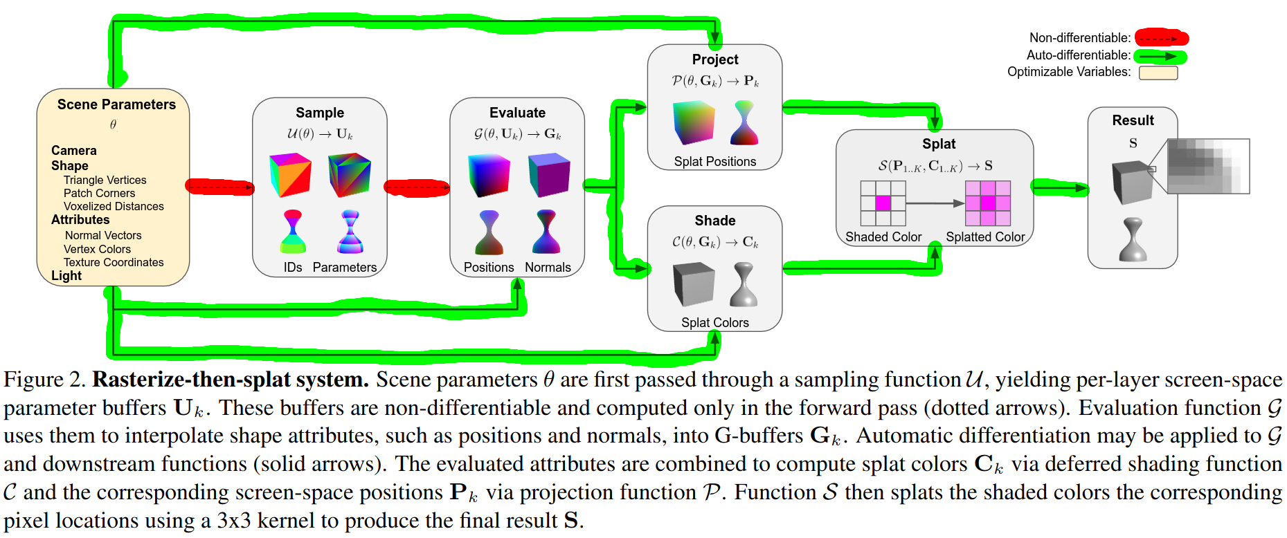
Going through the diagram we can see that we already have most of what we need to implement this in our codebase! Our rasterizer produces a triangle ID buffer and a barycentric coordinate buffer. This is the sampling process in the diagram. The evaluation process creates G-buffers for world position and normals. We have an attribute interpolator class that we have already used for just this purpose. The shading process produces a shaded color buffer just like our Blinn-Phong shader. The only things that we are missing are the processes for creating a splat position buffer and the splat buffer. Let’s now look at those more closely.
Splat Position Buffer
Recall the process of mapping triangle vertices from world space to screen space that takes place in our rasterizer. First, we take vertex coordinates in world space and project them into clip space using our camera view and projection matrices. Next, we perform perspective division to get NDC coordinates. Finally, we apply a viewport transform to get the screen space coordinates of each vertex. The splat position buffer can be computed in exactly the same way. We take each pixel in the world position buffer, and map the world coordinates to screen coordinates using the camera matrices and the viewport transform.
The splat position buffer is a bit strange because the values it contains are trivial. After all, the screen space coordinates of pixel \((x,y)\) are \((x,y)\). So why are we doing math to compute such an obvious value? The reason is that we need a path for gradients to flow from our final splat buffer to the scene paramters via AD. If we treat the splat positions as constant, we cut off the path for gradients. Remember that in this approach, the barycentric buffer is treated as a result of a non-differentiable sampling process. Therefore, the barycentric buffer is treated as constant. It’s important that we don’t also try to backpropagate gradients through the rasterizer when we use this approach or we will obtain incorrect gradients.
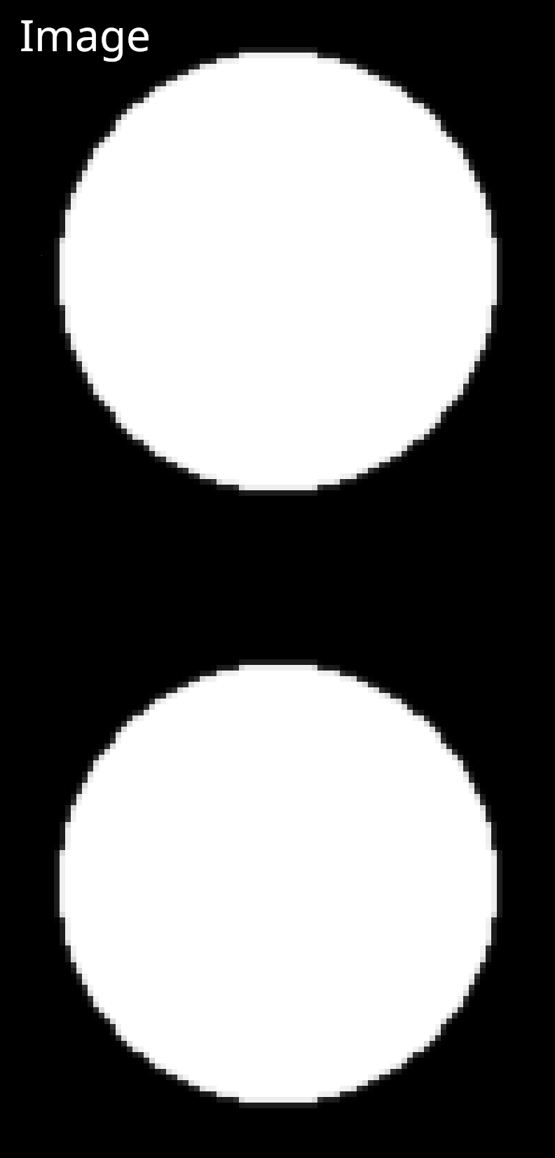
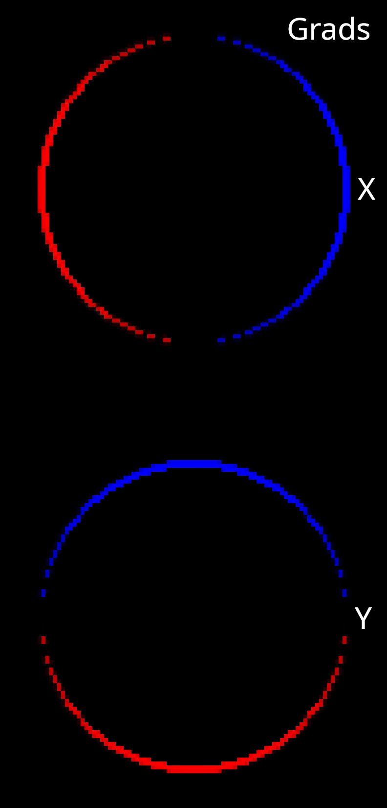
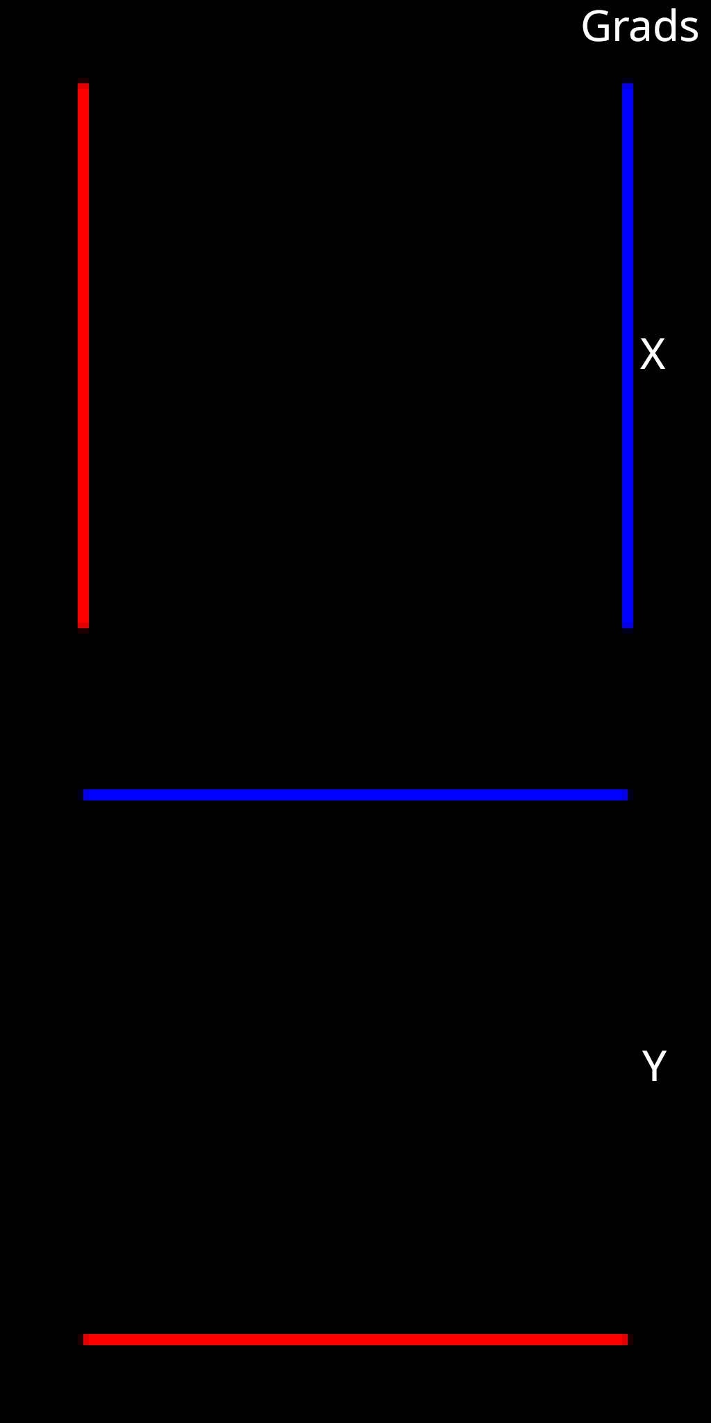
Below you can see the \(x\) and \(y\) components of an example splat position buffer. There may be small and inconsequential errors in the buffer due to floating point computation. Overall, the pixel values correspond almost exactly with the pixel coordinates.
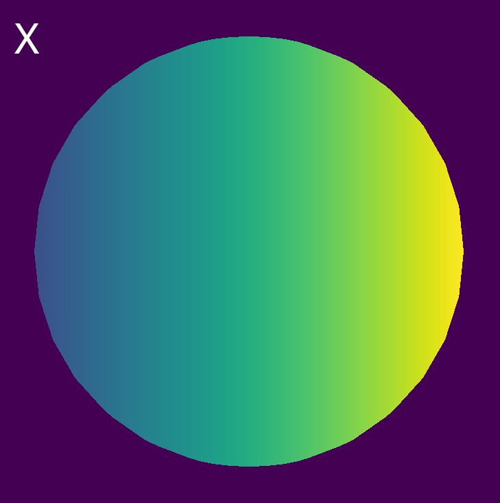
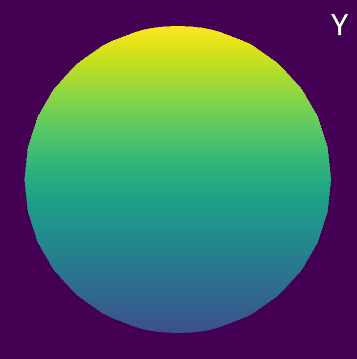
Now we know how to create a buffer that tells us where splats should be centered in an image. The buffer is also connected via AD to the camera and mesh vertex parameters.
Splat Buffer
The final step in the RTS approach is to splat the shaded pixel colors at the locations specified in the splat position buffer. The sole purpose of splatting is to solve the discontinuity problem by making hard, discontinuous boundaries into soft, continuous boundaries. Therefore, the splat kernel must be continuous and have support greater than one pixel. We would also like the splatted image to resemble the shaded image as much as possible. Therefore, the splatting operation should have a minimal effect on the image, and the kernel support should be as small as possible. The obvious choice given this description is a small Gaussian kernel with a 3x3 pixel support, although it is possible to use other kernels. In the RTS paper, a Gaussian kernel with \(\sigma = 0.5\) pixels is used. The formula used to compute the weight at pixel \(\mathbf{q}\) of a splat centered at pixel \(\mathbf{p}\) is shown below.
\begin{equation} w_\mathbf{p}(\mathbf{q}) = \frac{1+\epsilon}{W_\mathbf{p}} \cdot \text{exp} \Bigg( \frac{-|| \mathbf{q} - \mathbf{p} ||^2_2}{2\sigma^2} \Bigg) \end{equation}Using weights defined by this formula, each splat buffer pixel is computed as the weighted sum of the shaded colors of pixels in a 3x3 neighborhood. Here, \(W_\mathbf{p}\) is a normalization factor computed from the sum of a Gaussian kernel in a 3x3 neighborhood. The inclusion of this factor means that a full 3x3 neighborhood of weights will sum to \(1 + \epsilon\).
The Importance of Normalization
Now, you are probably asking yourself why that \(\epsilon\) term is in the weight equation. Having a full 3x3 neighborhood of weights sum to 1 would preserve the brightness of a shaded image. Surely this is what we want to do?
While we do want to preserve the brightness of the shaded image, there is a subtle problem with the splatting approach that we must adress somehow. Rasterization, as a sampling process, will always produce samples that are exactly 1 pixel apart in screen space. This is hard-coded into the forward process of our rasterizer. However, the splatting operation does not know anything about this. From the point of view of the splatting operation, the splat positions could move closer together, or further apart, and this would affect the pixel values in the splat image. If the splats spread out at a particular pixel, the image would become darker at that pixel. If the splats squish together at a particular pixel, the image would become brighter at that pixel. Here is a visualization of this phenomenon using Gaussian kernels in 2D to make things a bit clearer.
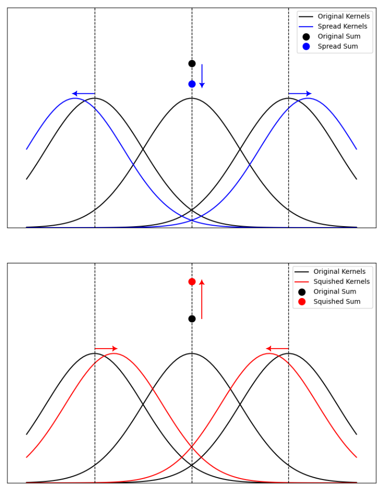
When AD is applied to the splatting operation, it may produce gradients that correspond to the spreading or squishing of splats. These gradients would be misleading and incorrect because splat positions are always separated by 1 pixel. Therefore, some method is required to prevent the AD system from computing gradients that correspond to splat spreading and squishing. This is where the \(\epsilon\) parameter comes into play.
The \(\epsilon\) parameter is set to a small positive value (0.05 in the RTS publication) so that a full 3x3 neighborhood of splat weights always sums to \(>1\). When the splatting operation is performed, the splat buffer pixel is computed as the weighted sum of the shaded colors of neighbor pixels. If the splat weight sum is \(>1\) an extra normalization step is performed where the weighted sum of colors is divided by the splat weight sum. This has the effect of removing those undesirable gradients, while preserving image brightness. If the splats were to squish together around a pixel, the splat weight sum increases and is incorporated into the normalization so that the pixel does not get brighter. Likewise, if the splats were to spread out around a pixel, the splat weight sum decreases and is incorporated into the normalization so that the pixel does not get darker.
For splats on silhouette boundaries, the splat weight sum is \(<1\) and the pixels are not normalized. This is important because we do need the gradients from splat squishing and spreading to be captured in those regions. In other words, boundary pixels do become brigher or darker as the silhouette boundary moves. If we were to normalize these pixels by the splat weight sum, we would not properly capture silhouette boundary gradients, and that is the whole point of applying RTS in the first place!
Single-Layer Splatting
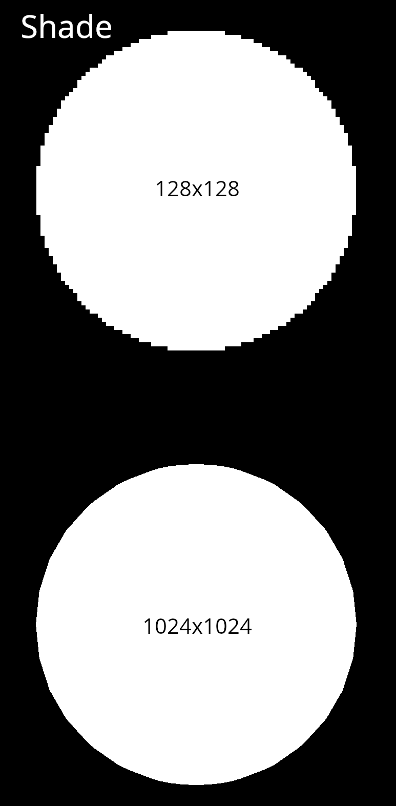
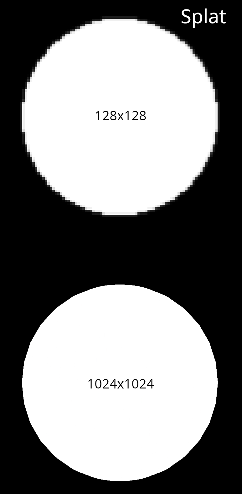
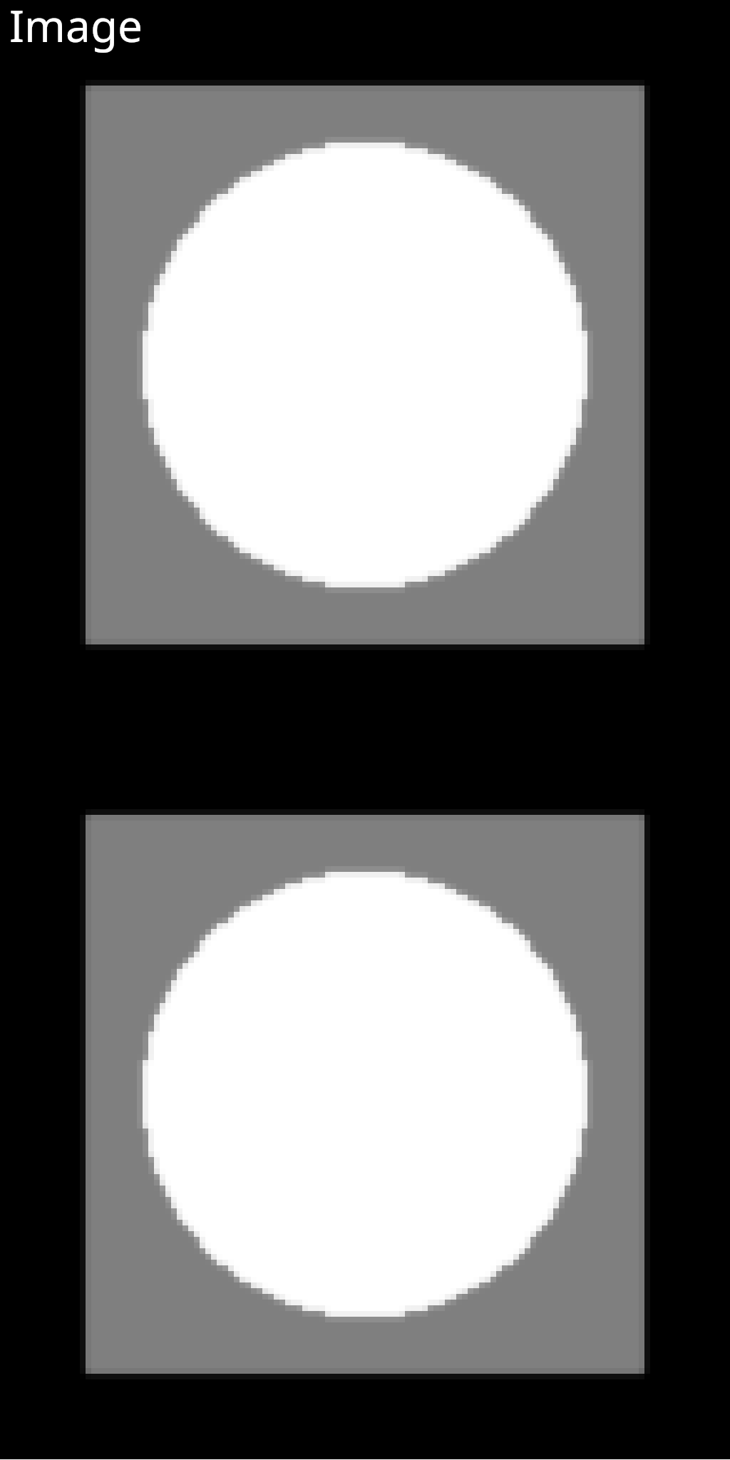
We have now described the two additional operations required to implement the RTS approach in our codebase! Let’s see what the results are. First we can compare a silhouette image with the splatted version of the same image. We can see by looking at the silhouette boundary that the splat buffer is a slightly blurred version of the shade buffer. This is apparent in low resolution images but nearly invisible in high resolution images.
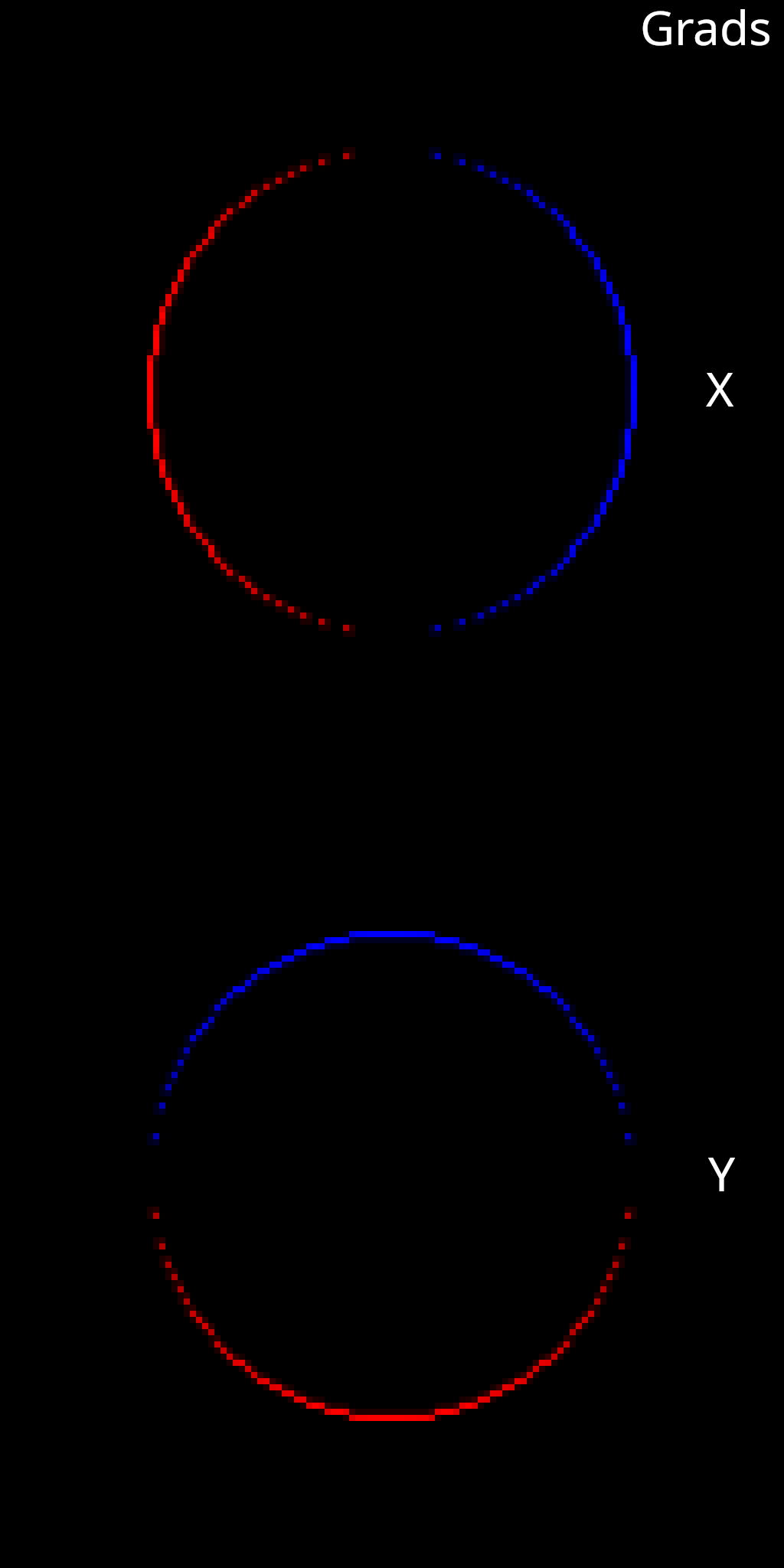
Next, let’s visualize a Jacobian image with respect to mesh translation to see if this has helped us to solve the discontinuity problem.
This looks much better than before! The boundary gradients are exactly what we would expect to see for a mesh translation. So far the RTS approach has succesfully solved the discontinuity problem.
Before we move on to using RTS in an inverse rendering task, there is one more experiment we need to run. The previous experiment showed that we were able to get correct gradients at a silhouette boundary against a background. But does RTS still work when a silhouette boundary is against another mesh in the scene? This is a known problem of previous approaches like DIB-R so we should probably check.
For this experiment we will place our sphere mesh in front of a simple plane mesh. We still wish to use silhouette shading, so we will shade the plane grey and the sphere white to ensure that there actually is a color differential in the shaded buffer We will start by repeating the previous experiment where we compute a Jacobian image with respect to x and y translations of the sphere.
That looks ok. Now, let’s try an experiment where we compute a Jacobian image with respect to x and y translation of the grey plane mesh.
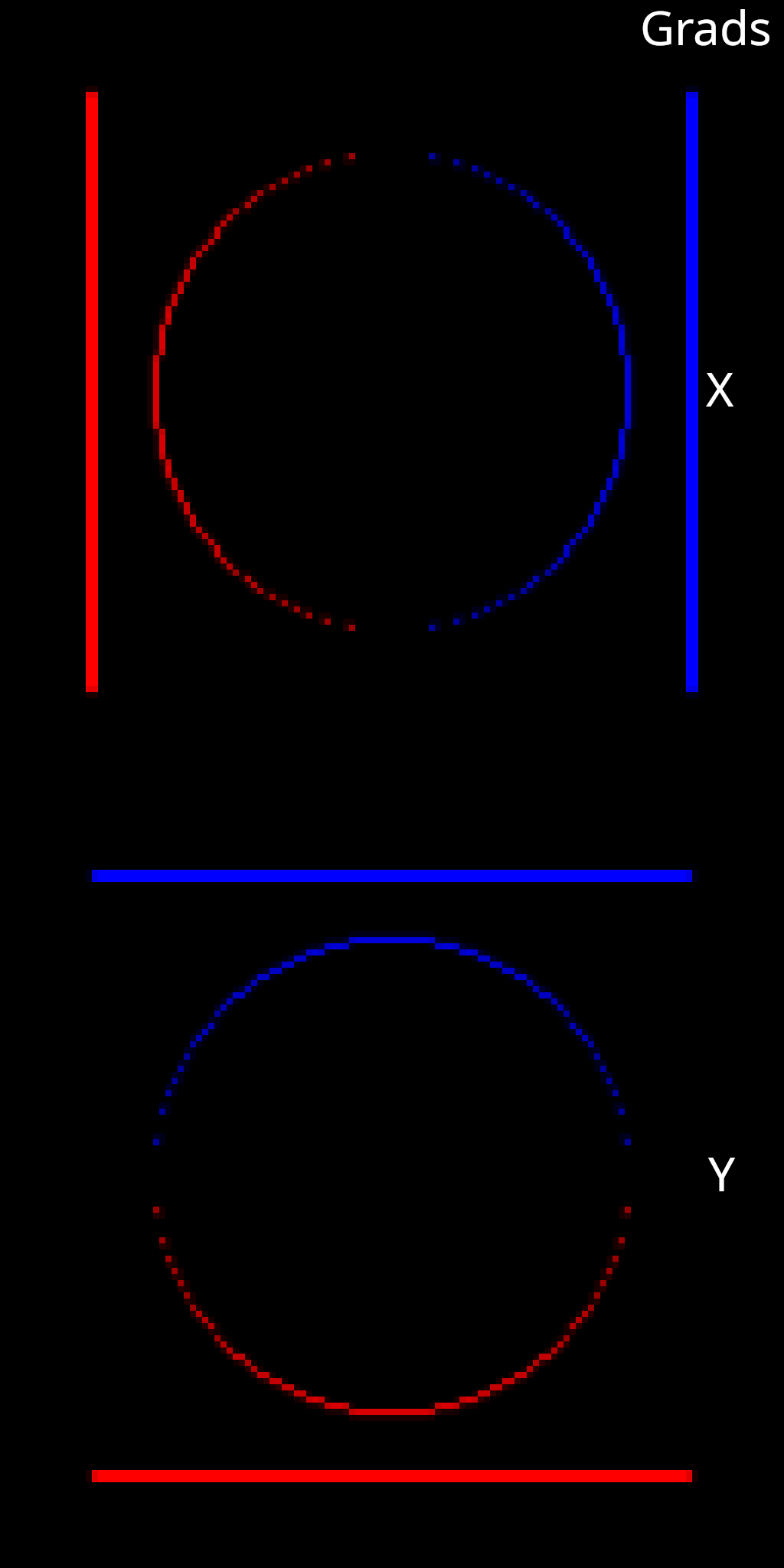
Now it appears that we do have a problem. The gradients at the outer boundary of the plane look good. But why are we seeing non-zero gradients around the sphere boundary? As the plane translates behind the sphere, we wouldn’t expect the pixel values at the boundary of the sphere to change at all. Can you think of what might be going wrong here?
The answer comes back to the normalization that we just discussed. Consider a pixel right on the silhouette boundary between the white sphere and the grey plane. Let’s take a white pixel on the sphere as an example. As a neighboring grey pixel translates towards the white pixel, due to the underlying translation of the plane mesh, the splat weight of the grey pixel increases. This pixel will be normalized, and after normalization, the pixel becomes slightly more grey (darker). Likewise, if a neighboring grey pixel translates away from the white pixel, due to the underlying translation of the plane mesh, the splat weight of the grey pixel decreases. After normalization, this results in the splat pixel becoming slightly more white (brighter). However, this is not what should happen. What should happen is that the grey pixel of the plane should slide behind the white pixel of the sphere, leaving the white pixel unchanged.
In short, the RTS approach doesn’t normalize at silhouette boundaries against background pixels, therefore, it should also not normalize at silhouette boundaries against other mesh pixels. In order to solve this problem, we must adapt the splatting operation to be aware of multiple depth layers.
Multi-Layer Splatting
In order to properly handle silhouette boundary gradients agianst other mesh pixels, the RTS approach uses a 3 layer accumulation buffer for splats. For a pixel \(\mathbf{p}\) being splatted at pixel \(\mathbf{q}\), the 3 layers correspond to splatting behind the surface at \(\mathbf{q}\) (layer \(\text{S}^-\)), splatting in front of the surface at \(\mathbf{q}\) (layer \(\text{S}^+\)), and splatting coincident with the surface at \(\mathbf{q}\) (layer \(\text{S}^\circ\)).
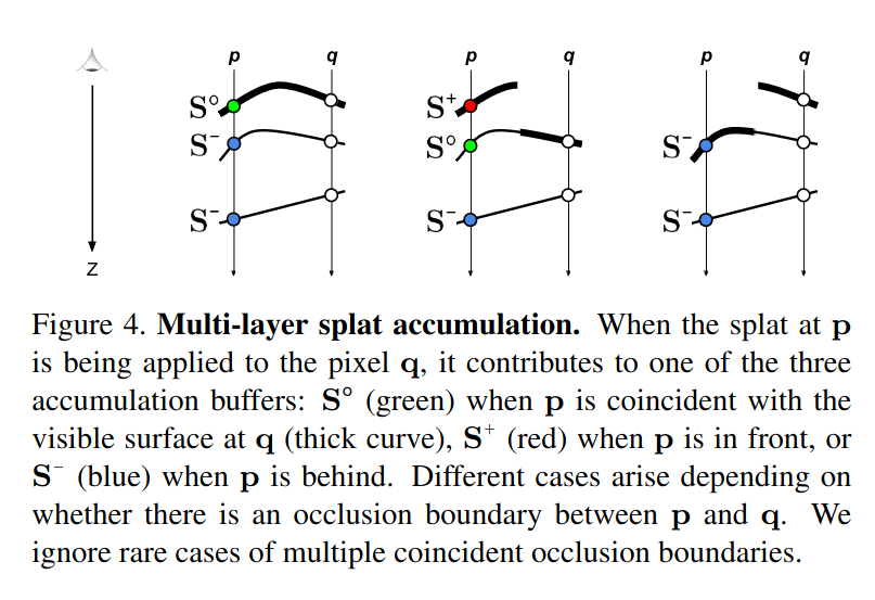
The multi-layer splatting operation proceeds slightly differently from the single layer approach described above. First, pixels are splatted in their 3x3 neighborhood into the three splat accumulation layers. Next, each splat accumulation layer is normalized separately. Finally, the layers are composited to produce the final output buffer.
Occlusion Estimation
The question now is how to determine which splat accumulation layer each splat should be placed in. This is not trivial, as our mesh could have many different sillhouette boundaries at different depths in the image. A simple depth thresholding method is not likely to be robust. This is where the multi-layer rasterization approach that we implemented earlier comes in handy. Recall that our shade buffer, and our depth buffer actually have two layers.
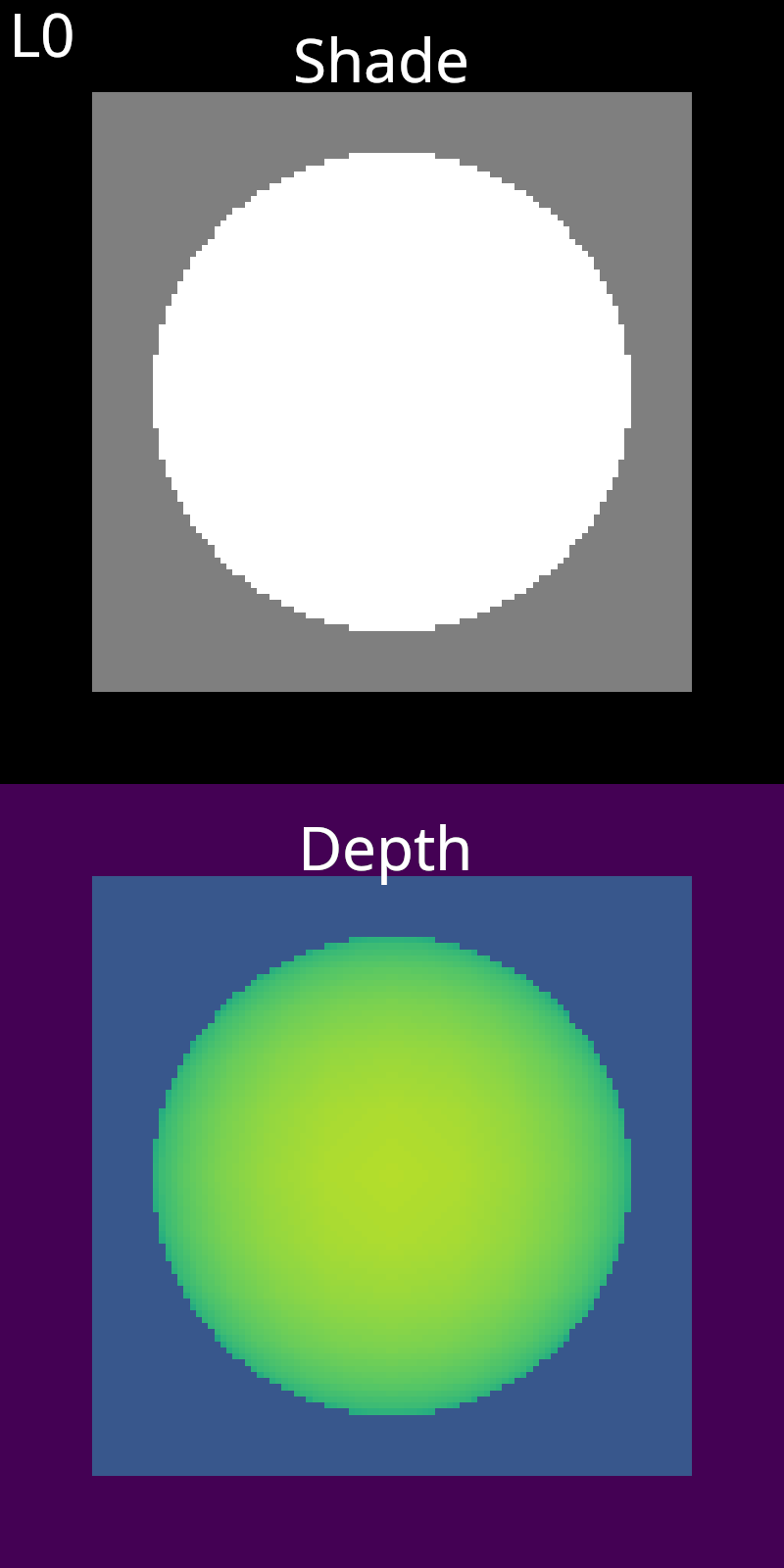
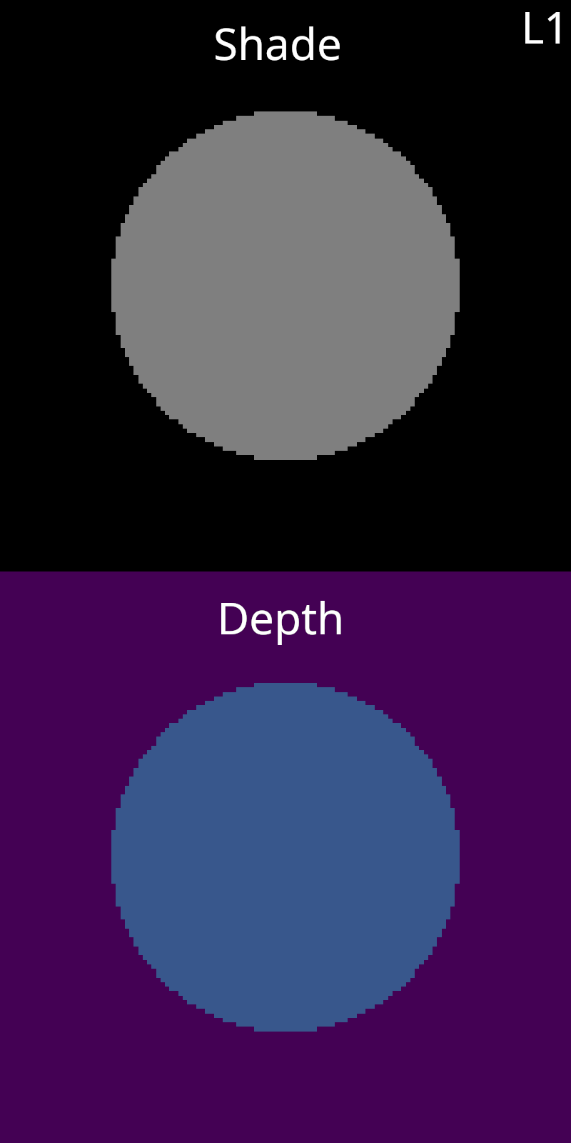
We can use this information to determine the occlusion relationship between neighboring pixels. To do this for a pair of pixels, we compare the difference in depth between the first layer of each pixel (\(d_{00}\)), and the differences in depth between the first and second layers of each pixel (\(d_{01}, d_{10}\)). If the second layer of either pixel is empty, the distances associated with it are treated as infinite. Here is a quick diagram to make this clear.
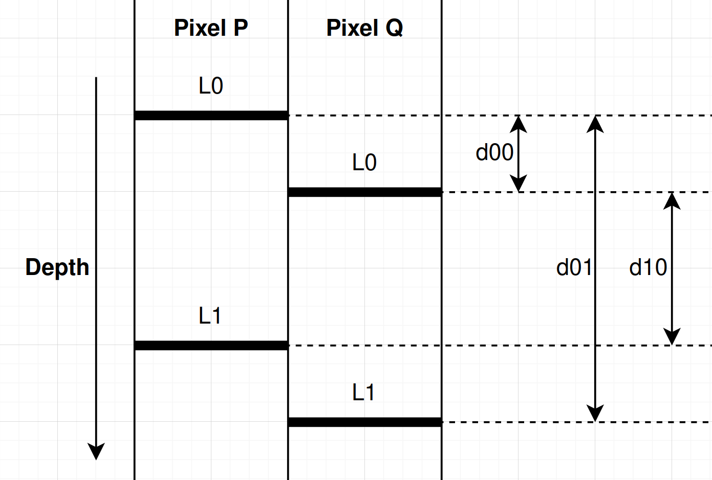
For neighbor pixels \(\mathbf{p}\) and \(\mathbf{q}\), if \(d_{00}\) is the smallest value, then neither pixel occludes or is occluded by the other. If \(d_{10}\) is the smallest value, then pixel \(\mathbf{p}\) occludes pixel \(\mathbf{q}\). If \(d_{01}\) is the smallest value, then pixel \(\mathbf{q}\) occludes pixel \(\mathbf{p}\).
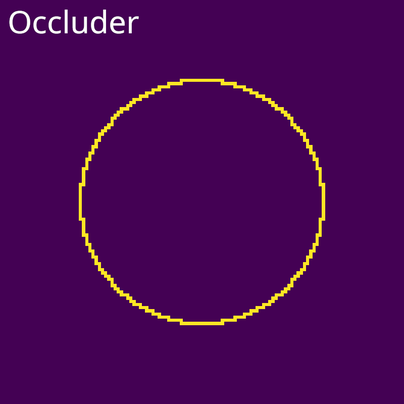
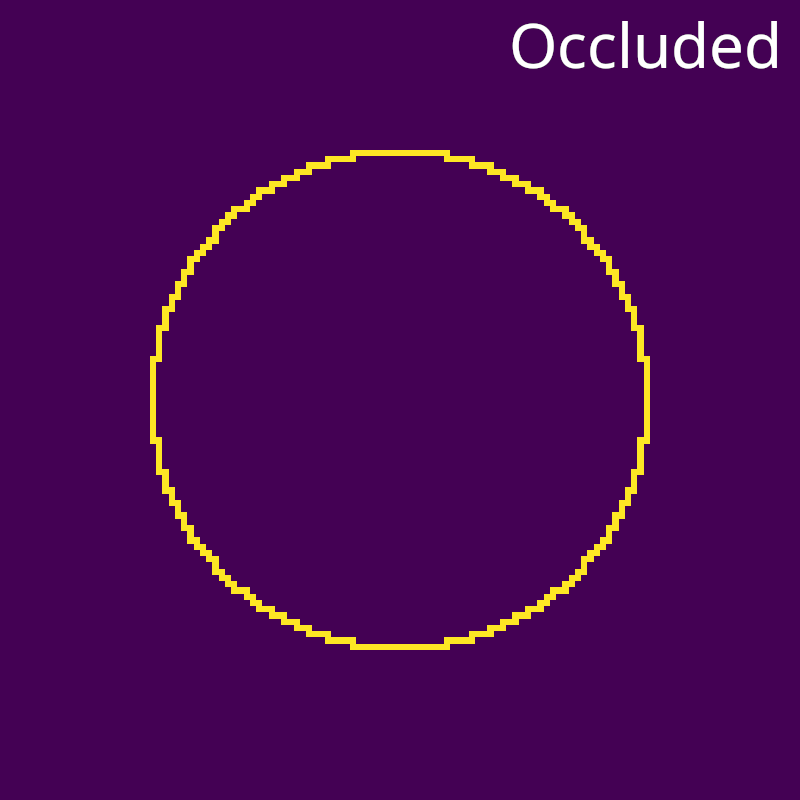
In our implementation, we compute two buffers to capture this occlusion information. The occluder buffer is 1 for pixels that occlude any neighbor pixel and 0 othewise. The occluded buffer is 1 for pixels that are occluded by any neighbor pixel and 0 othewise. This approach ignores rare cases of mutiple coincident occlusion boundaries. For the RTS approach, the occlusion buffers do not capture occlusions against background pixels because background pixels are not splatted. Here are the buffers for our running example.
Results
Returning the the splatting operation, we can now use the occlusion buffers above to determine in which accumulation layer to place each splat. Let’s again consider a pixel \(\mathbf{p}\) being splatted onto neighbor pixel \(\mathbf{q}\). If \(\mathbf{p}\) is an occluder and \(\mathbf{q}\) is occluded, the first layer of \(\mathbf{p}\) is splatted into \(\text{S}^+\) and the second into \(\text{S}^\circ\). If \(\mathbf{p}\) is occluded and \(\mathbf{q}\) is an occluder, the first and second layer of \(\mathbf{p}\) are splatted into \(\text{S}^-\). Otherwise, the first layer of \(\mathbf{p}\) is splatted into \(\text{S}^\circ\) and the second into \(\text{S}^-\). Here are the resultant splat weights of each accumulation buffer using our running example.

Finally, let’s re-run the experiment that propted this multi-layer splat formulation. Once again, we create a Jacobian image with respect to the translation of the plane mesh that is behind a sphere mesh. This time, we hope to see that the spurious gradients around the sphere mesh are gone.
Perfect! This is exactly what we would expect to see as the plane mesh moves behind the sphere. The boundaries of the plane change, and no change is observed around the boundaries of the sphere. The multi-layer approach has solved our issue.
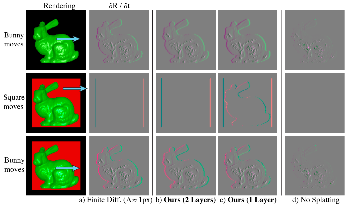
The Jacobian images that we have been generating for our running example of a sphere in front of a plane, have effectively replicated the results from Figure 3 of the RTS publication. As mentioned earlier, Jacobian images are a very helpful way to visualize gradients for differentiable rendering algorithms. You will find them in most papers on differentiable rendering so it is important to be able to understand and create them.
Coding Challenge 8
The coding challenge for this lesson is to implement the RTS approach and generate some Jacobian images to confirm that the boundary gradients are working properly. Some additional discussion about our implementation can be found below. You can also go look at the project codebase to see exactly how our implementation works.
Implementation
Splat Position Interpolator
The first class that we have for the RTS approach computes the screen space coordinates used to define splat positions. This class uses a world space buffer, and a camera to process each pixel. We also reference a triangle id buffer (to identify pixels that are empty). The single kernel associated with this class parallelizes over all pixels, and applies a series of transformation used to map from world space to screen space. The output is another image buffer that contains screen space coordinates.
@ti.data_oriented
class TriangleSplatPositionInterpolator:

    def __init__(
        self,
        camera: Camera,
        world_space_buffer: ti.Vector.field,
        triangle_id_buffer: ti.Vector.field,
    ):
        self.camera = camera
        self.world_space_buffer = world_space_buffer
        self.triangle_id_buffer = triangle_id_buffer

        self.screen_space_buffer = ti.Vector.field(
            n=2, dtype=float, shape=self.world_space_buffer.shape, needs_grad=True
        )

        self.x_resolution = triangle_id_buffer.shape[0]
        self.y_resolution = triangle_id_buffer.shape[1]

    def forward(self):
        self.clear()
        self.interpolate()

    def backward(self):
        self.interpolate.grad()

    def clear(self):
        self.screen_space_buffer.fill(0)
        self.screen_space_buffer.grad.fill(0)

    @ti.kernel
    def interpolate(self):
        for x, y, l in self.screen_space_buffer:
            pass # Your code here
Occlusion Estimator
To support multi-layer splatting, we implemented a separate class to handle occlusion estimation. This class references a depth buffer and also a triangle id buffer to check if pixels are empty. The forward method populates two binary mask buffers that indicate which pixels are occluded and which pixels are occluders. The occlusion estimator does not require a backward method and the fields do not have gradients. Occlusion is treated as a constant during backpropagation.
@ti.data_oriented
class OcclusionEstimator:

    def __init__(
        self,
        depth_buffer: ti.Vector.field,
        triangle_id_buffer: ti.field,
    ) -> None:

        self.depth_buffer = depth_buffer
        self.triangle_id_buffer = triangle_id_buffer

        self.x_resolution = depth_buffer.shape[0]
        self.y_resolution = depth_buffer.shape[1]

        self.is_occluded_buffer = ti.field(
            dtype=int, shape=(self.x_resolution, self.y_resolution)
        )
        self.is_occluder_buffer = ti.field(
            dtype=int, shape=(self.x_resolution, self.y_resolution)
        )

    def forward(self):
        self.clear()
        self.compute_occlusions()

    def clear(self):
        self.is_occluded_buffer.fill(0)
        self.is_occluder_buffer.fill(0)

    @ti.kernel
    def compute_occlusions(self):
        for x, y in ti.ndrange(self.x_resolution, self.y_resolution):

            # Iterate over a 3x3 neighborhood
            for l in range(3):
                for m in range(3):
                    pass # Your code here
Splatter
The final and most complicated class is the splatter. This class references a shade buffer, and the screen space buffer that defines splat positions. This class also references a depth buffer that is passed to an occlusion estimator, and a triangle id buffer to check for empty pixels.
There are two kernels associated with this class and three image buffers. The first kernel performs the actual splating operation, referencing the occlusion estimator to determine the appropriate splat layer. This kernel populates the splat accumulation buffers as well as a buffer that stores the accumulated splat weights. Both of these buffers have three layers. The second kernel performs splat normalization and, finally, composites \(S^+\) over \(S^\circ\) over \(S^-\) to produce the output buffer.
@ti.data_oriented
class TriangleSplatter:

    def __init__(
        self,
        shade_buffer: ti.Vector.field,
        screen_space_buffer: ti.Vector.field,
        depth_buffer: ti.Vector.field,
        triangle_id_buffer: ti.Vector.field,
        kernel_variance: float = 0.25,
        adjustment_factor: float = 0.05,
    ):

        self.shade_buffer = shade_buffer
        self.screen_space_buffer = screen_space_buffer
        self.depth_buffer = depth_buffer
        self.triangle_id_buffer = triangle_id_buffer
        self.kernel_variance = kernel_variance
        self.x_resolution = shade_buffer.shape[0]
        self.y_resolution = shade_buffer.shape[1]

        self.occlusion_estimator = OcclusionEstimator(
            depth_buffer=depth_buffer, triangle_id_buffer=triangle_id_buffer
        )

        self.splat_buffer = ti.Vector.field(
            n=3,
            dtype=float,
            shape=(self.x_resolution, self.y_resolution, 3),
            needs_grad=True,
        )

        self.splat_weight_buffer = ti.field(
            dtype=float,
            shape=(self.x_resolution, self.y_resolution, 3),
            needs_grad=True,
        )

        self.output_buffer = ti.Vector.field(
            n=3,
            dtype=float,
            shape=(self.x_resolution, self.y_resolution),
            needs_grad=True,
        )

        # Pre-compute normalization constant for gaussian splats
        kernel_sum = 0.0
        for u in [-1, 0, 1]:
            for v in [-1, 0, 1]:
                d_squared = u**2 + v**2
                kernel_sum += exp(-d_squared / (2.0 * kernel_variance))
        self.normalization_constant = (1.0 + adjustment_factor) / kernel_sum

    def forward(self):
        self.clear()
        self.occlusion_estimator.forward()
        self.splat()
        self.normalize_and_composite()

    def backward(self):
        self.normalize_and_composite.grad()
        self.splat.grad()

    def clear(self):
        self.splat_weight_buffer.fill(0)
        self.splat_buffer.fill(0)
        self.output_buffer.fill(0)
        self.splat_buffer.grad.fill(0)
        self.splat_weight_buffer.grad.fill(0)
        self.output_buffer.grad.fill(0)

    @ti.kernel
    def splat(self):
        for x, y, l in self.shade_buffer:
            if self.triangle_id_buffer[x, y, l] != 0:

                # Grab the splat location and color
                splat_location = self.screen_space_buffer[x, y, l]
                splat_color = self.shade_buffer[x, y, l]

                # Splat over the 3x3 neighborhood
                for i in ti.static(range(3)):
                    for j in ti.static(range(3)):
                        pass # Your code here

    @ti.kernel
    def normalize_and_composite(self):
        for x, y in ti.ndrange(self.x_resolution, self.y_resolution):
            pass # Your code here

    @ti.func
    def splat_weight(self, d_squared: float) -> float:
        return (
            tm.exp(-d_squared / (2.0 * self.kernel_variance))
            * self.normalization_constant
        )
Conclusion
In this lesson, we covered the RTS approach to solving the discontinuity problem. We saw how Gaussian splatting can be used to turn hard discontinuous boundaries into soft continuous boundaries. We reviewed several tricks that are required to make this approach viable. This included a method for splat normalization, and a method for multi-layer splatting. In the next lesson, we will look at another method for solving the discontinuity problem based on distance-to-edge antialiasing.