3) Rasterization
Welcome back and buckle up! In this lesson, we are going to implement a 3D triangle mesh rasterizer.
Rasterization is not a simple algorithm and can be quite challenging to implement. It is ammenable to parallelization, but is not embarassingly parallelizable like ray tracing. Packages like PyTorch3D, Tensorflow Graphics, and Kaolin, implement rasterization with custom C++ and CUDA kernels (and matching custom gradient kernels). Using Taichi, we will implement a parallelized, cross-platform, triangle rasterizer, without writing a line of C++, CUDA or any custom gradient code.
Contents
Discussion
Software vs. Hardware Rasterization
Let’s begin by talking about GPUs. With all of the chatter around AI in recent years, some people may have forgotten that the acronym GPU stands for graphics processing unit. These specialized pieces of computing hardware were originally developed for graphics applications and not machine learning. It was not until 2007, when Nvidia introduced CUDA, that the programable components of GPUs began being widely used for general purpose computing. This implies that there are other, non-programable components in GPUs. These components, sometimes called fixed-function resources, are what were originally used to implement the graphics pipeline including algorithms like rasterization.
There are several advantages to using fixed-function hardware to implement graphics algorithms, the main one being performance. GPU manufacturers have designed highly specialized and extremely efficient hardware components for different aspects of the graphics pipeline. These components are exposed for application and game developers to use (with some degree of configurability) through device specific drivers. In order to enable developers to write cross-platform code that works with many different types of graphics hardware, application programming interfaces (APIs) were developed as an additional abstraction layer on top of device drivers. Some of the most popular graphics APIs today are OpenGL, Vulkan, DirectX, OptiX, and Metal. Many of your favorite games and graphical applications make use of these APIs.
Since CUDA was released in 2007, there has been hardware innovation at an incredible pace. GPUs have proven to be extremely useful for many non-graphics applications, ML most notably. The reason is that GPUs enable many different parts of a computation to be performed at the same time (in parallel). Depending on what computation is being performed, this can result in enormous improvements in performance. The programable components of GPUs have grown more, and more powerful, such that it is no longer a crazy idea to implement the entire graphics pipeline in software using the programmable components of GPUs. It is still difficult to compete with the performance of fixed-function hardware, but fully programmable graphics pipelines have the advantage of flexibility. Developers working on software graphics pipelines can explore different algorithms and edit their pipelines with complete freedom.
In this lesson, we will be implementing a rasterizer completely in software. This allows us greater ability to edit and explore the rasterization algorithm. This will also provide much better educational content, for no part of our algorithm will be hidden behind opaque API calls. Our implementation will not perform on par with hardware rasterization, but it won’t be too shabby either.
Deferred Shading
Rasterization computes which geometry elements (triangles in this case) intersect the rays associated with each pixel in an image (often called primary or camera rays). Rays are defined by an origin and a direction vector in 3D space. Rasterization also determines how triangles occlude one another when multiple triangles are intersected by a primary ray (a process called Z-buffering). However, this alone is not sufficient to render a final image. It still remains to determine the color of each pixel (a process called shading). In regular rendering applications, shading and rasterization computation can be performed at different times throughout the pipeline, typically optimized for performance. In differentiable rendering applications, shading often takes place after rasterization using an approach called deferred shading.
In a deferred shading approach, the rasterization process outputs image buffers that contain information related to triangle coverage and occlusion. Subsequent processing stages then compute additional buffers, called G-buffers, containing information related to geometry and texture. Finally, a shading computation is performed that uses the G-buffers to compute a final color at each pixel. Therefore, when implementing a differentiable rasterizer, we must output buffers that provide sufficient information to support downstream shading operations. We must also ensure that gradients on relevant buffers can be backpropagated to the inputs of the rasterizer.
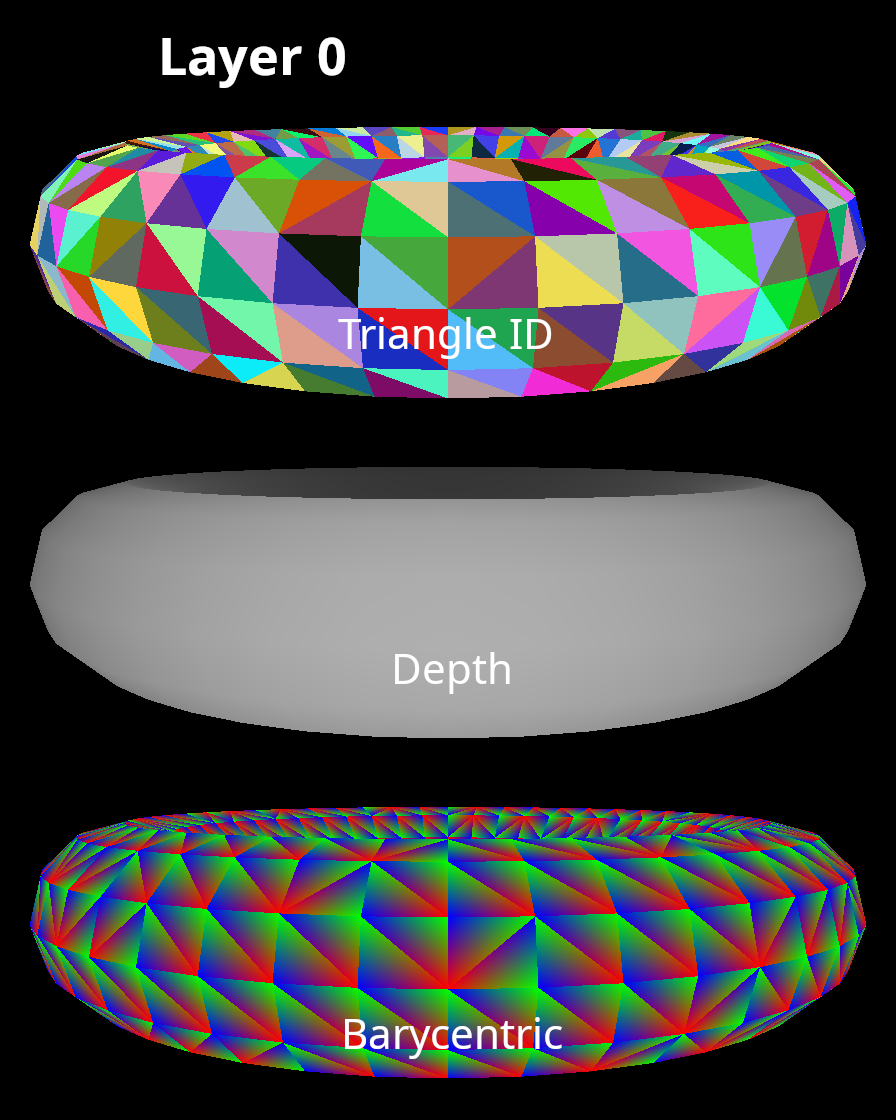
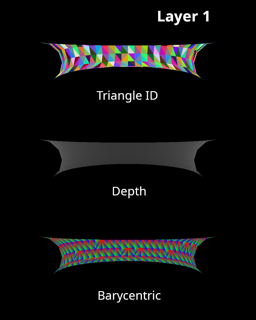
Commonly, differentiable rasterizers output three buffers, only one of which requires gradients. A triangle id buffer contains information about which triangle (if any) is visible at each pixel in the image. A depth buffer contains information about how far the visible triangle is from the camera. Finally, a barycentric coordinate buffer contains information about exactly which point on each triangle is visible at the center of each pixel. The barycentric coordinate buffer is the buffer that must support gradient backpropagation.
Multi-layer Rasterization
During the Z-buffering stage of the rasterization algorithm, we typically only keep track of the triangle that is closest to the camera at each pixel in the image. However, there are certain applications in which it is useful to keep track of more than one layer. One of these applications is rendering meshes that are partially transparent. In this scenario, it is also necessary to know what triangles are behind partially transparent triangles.
In one of the differentiable rasterization approaches that we will be implementing, it is necessary to keep track of two layers during rasterization. Thankfully, this is not a difficult thing to implement. Each output buffer will have two layers, and, during Z-buffering, we will simply keep track of the two closest triangles instead of just one. For more detail on muli-layer rasterization, here is a good presentation from researchers at Nvidia.
The Half-Plane Algorithm
There are many different, creative approaches for implementing rasterization. The half-plane approach, which we will be using, was originally proposed by Juan Pineda in 1988, and many improvements have been made since then. The reason that this algorithm is very popular is because it allows for many pixels to be processed in parallel. More parallelism means that things run faster on GPUs (broadly speaking).
The core idea behind the half-plane algorithm is that triangles can be described by three edges. For each edge, we can define a linear function that, based on the sign of the function, tells us which side of the edge a point is on. Therefore, for any point, we can evaluate three linear functions to determine if the point is inside or outside of a triangle. We can also use edge function values to compute barycentric coordinates. Barycentric coordinates allow us to easily interpolate depth and any other per-vertex attribute of interest. The ryg blog, scratch a pixel, and tiny renderer projects all have excellent content that introduce the half-plane algorithm from first principles.
Fixed vs. Floating Point Edge Functions
One additional point that is important to discuss is the role of fixed point (or integer) representations in rasterization algorithms. Fixed-function GPU rasterizers use integer data types to represent vertex coordinates during rasterization. After being mapped to screen space, vertices are snapped to a fine grid (typically with sub-pixel precision) and converted to integer data types. This may seem strange at first, but it is actually a very good idea. One reason for doing this is that integer artethmitic is faster on most hardware. Another reason is that floating point rasterizers often suffer from precision issues. This may seem backwards at first if you have never learned about how floating point numbers are represented in computers. It’s not something that I will detail here, but there are some good blogs that discuss the numerous tricks and pitfalls of floating point numbers. If you try to implement a floating point rasterizer, you will probably encounter cracks that appear between triangles. Furthermore, floating point numbers can cause issues if you want to properly implement rasterization fill rules, which we will. The scratch a pixel blog has a good discussion on integer coordinates in rasterizers. The ryg blog also has a good discussion of fill rules and the use of integer coordinates.
One of the downsides of using integer coordinates is that they can cause integer overflow. Integer data types have min and max values that can be exceeded when performing rasterization, leading to undesirable behaviour. For this reason, rasterization pipelines typically have clipping stages for the purpose of preventing integer overflow. In our codebase, we do not implement clipping. This is because it is relatively complicated, not particularly interesting, and is tangential from our primary goal of explaining and implementing differentiable rasterization. For most applications of differentiable rendering, and for all of the examples that we explore, the objects being rendered are in front of the camera, and do not require clipping. We also use some well known tricks that give us plenty of room in our integer variables to fit large triangles with sub-pixel precision.
Rasterization Algorithm
Now that we understand the foundational concepts of rasterization, we are ready to think about the overall structure of the algorithm. In our codebase, we will follow a simplified version of the algorithm described in the 2011 paper High-Performance Software Rasterization on GPUs by Nvidia researchers Laine and Karras. Here is an overview figure from that paper.
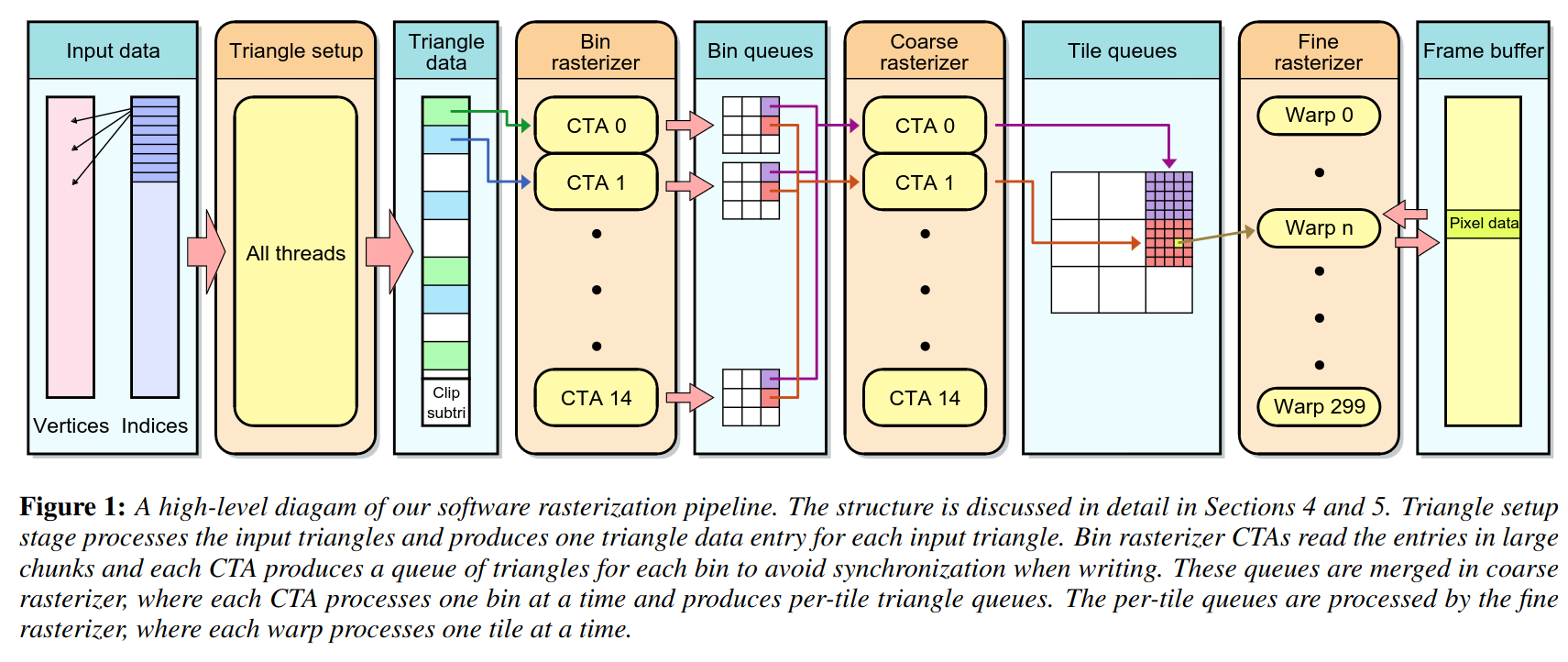
Let’s break it down in simple terms. There are four stages to their algorithm. The main reason for using multiple stages is to maximize the amount of processing that can take place in parallel. Again, more parallelism means that things run faster on GPUs (broadly speaking). As mentioned earlier, rasterization is interesting because some parts of the algorithm can be performed in parallel, while other parts of the algorithm must be performed in sequence because they depend on results from earlier parts of the algorithm.
The first stage is called triangle setup. In this stage, all triangles are processed in parallel and the output is a data structure containing all triangle information that is required for future stages. The essential information for a setup triangle includes the edge functions (used to evaluate whether a pixel is inside a triangle) and the depth parameters (used for Z-buffering). The next two stages are bin and coarse rasterization. The goal of these stages is to prepare triangle processing queues for each 8x8 pixel tile in the image. A triangle is added to a tile queue if it overlaps part of the tile. The final stage is fine rasterization. Fine rasterization uses triangle edge functions to determine if a pixel is within a triangle. The fine rasterization stage also performs Z-buffering. If a pixel is inside a triangle, the depth at the pixel is evaluated and checked against the depth buffer to see if the triangle is occluded at that pixel. In the fine rasterization stage, each tile is processed in parallel and, within each tile, the triangles in the tile queue are processed sequentially. The reason for this is that Z-buffering requires information about previously processed triangles. Therefore, the triangles must be processed in sequence, and the image is divided into tiles so that many such processes can occur in parallel.
The algorithm we implement is slightly different.
Our rasterizer takes into account the fact that we are using a computing framework with automatic differentiation support, and we will not be implementing custom gradients.
Our rasterizer also does not enforce a consistent triangle rendering order.
This does not have any seriously concequences for our application, and makes the process of enqueueing triangles into tiles considerably simpler (we do not need bin and coarse rasterization stages).
Our rasterizer has four stages which are implemented as four separate Taichi kernels.
The first stage is called vertex_setup and all vertices are processed in parallel.
In this stage, the triangle vertices are transformed from world space to clip space according using a camera model as described in the previous lesson.
This kernel is differentiable and will be involved in the backward pass.
The second stage is triangle_setup, and it processes all triangles in parallel.
This kernel performs all triangle setup computations, and also adds the processed triangles into tile queues in preparation for the next stage.
This kernel is not involved in the backward pass and is not differentiable.
The third stage is rasterize, and each tile is processed in parallel.
This kernel computes pixel coverage for each triangle and also performs Z-buffering.
This kernel is also not involved in the backward pass and is not differentiable.
The final stage is called compute_barycentrics, and each pixel is processed in parallel.
This kernel computes the barycentric coordinates for each pixel.
This kernel is differentiable and is involved in the backward pass.
Gradient Flow
Notice that there are only 2 kernels involved in the backward pass.
Our implementation isolates the parts of the algorithm that require gradients by using separate kernels.
The compute_barycentric.grad kernel backpropagates gradients from the barycentric image buffer to the clip vertices intermediate data field.
The setup_vertices.grad kernel backpropagates gradients from the clip vertices to the camera matrices and to the mesh vertices.
It is also important to note that, even though this rasterizer supports gradients with respect to barycentric coordinates, we have not yet solved the discontinuity problem. This will become crystal clear in future lessons when we look at the backward pass in more detail and create some images to visualize gradients. For now, just keep in mind that our approach takes the backward pass into consideration.
Interactive Rasterizer
In addition to rendering static scenes, we implemented an interactive rendering demo. This provides a nice way to play around with the rasterizer using different camera positions and different meshes. Taichi has a very nice GUI system to visualize image-like fields. In order to create this demo, we wrote an additional camera controller class that updates camera parameters based on keyboard input. This demo also validates our implementation of the continuous camera parameterization from the last lesson. We are able to explore the full range of camera rotation without ever hitting a discontinuity in the representation space.
Here is a clip recorded on a computer with a 2070 super Nvidia GPU using a dragon mesh that has ~250k triangles (obtained from the Stanford 3D scanning repository). The framerate stays well above 60fps at a resolution of 1024x1024 pixels. We’re a few multiples away from harware rasterization performance, but we’re still doing pretty well!
Performance Profiling
We can also get a more detailed performance breakdown using Taichi’s profiling tools. The experiment below uses the dragon mesh that was shown above and runs forward and backwards on the rasterizer 1000 times. The profiler measures how much time each part of the program takes.
[Taichi] Starting on arch=cuda
=========================================================================
Kernel Profiler(count, default) @ CUDA on NVIDIA GeForce RTX 2070 SUPER
=========================================================================
[      %     total   count |      min       avg       max   ] Kernel name
-------------------------------------------------------------------------
[ 27.74%   2.448 s   1000x |    2.258     2.448     3.486 ms] vertex_setup_c87_0_reverse_grad_kernel_0_range_for
[ 17.59%   1.553 s   1000x |    1.538     1.553     1.923 ms] compute_barycentrics_c93_0_reverse_grad_kernel_0_range_for
[ 13.34%   1.177 s   1000x |    1.155     1.177     1.372 ms] rasterize_c90_0_kernel_0_range_for
[  9.47%   0.836 s   1000x |    0.798     0.836     1.017 ms] triangle_setup_c88_0_kernel_0_range_for
[  8.80%   0.777 s   1000x |    0.768     0.777     1.074 ms] compute_barycentrics_c92_0_kernel_0_range_for
[  5.66%   0.499 s   1000x |    0.470     0.499     0.762 ms] clear_c84_0_kernel_4_range_for
[  5.44%   0.480 s   1000x |    0.449     0.480     0.765 ms] clear_c84_0_kernel_1_range_for
[  5.34%   0.471 s   1000x |    0.444     0.471     0.756 ms] clear_c84_0_kernel_0_range_for
[  5.30%   0.467 s   1000x |    0.441     0.467     0.576 ms] clear_c84_0_kernel_2_range_for
[  0.56%   0.050 s   1000x |    0.007     0.050    15.458 ms] clear_c84_0_kernel_5_range_for
[  0.40%   0.035 s   1000x |    0.006     0.035     0.666 ms] clear_c84_0_kernel_6_gc_zero_fill
[  0.14%   0.012 s   1000x |    0.010     0.012     0.209 ms] vertex_setup_c86_0_kernel_0_range_for
[  0.09%   0.008 s   1000x |    0.005     0.008     0.118 ms] clear_c84_0_kernel_3_range_for
[  0.06%   0.005 s   1000x |    0.004     0.005     0.207 ms] clear_c84_0_kernel_6_gc_gather_list
[  0.05%   0.005 s   1000x |    0.003     0.005     0.287 ms] clear_c84_0_kernel_6_gc_reinit_lists
This result shows that roughly 27% of the time is spent in the vertex_setup.grad kernel, 18% is spent in the compute_barycentrics.grad kernel, 13% is spent in the rasterize kernel, and all other kernels take less than 10% of the total runtime.
We can also switch the backend to CPU and see how the performance changes.
Unsurprisingly, the CPU backend runs slower than the GPU backend.
Additionally, the processes that take the most amount of time are different.
On the CPU, 17% of time is spent on the triangle_setup kernel, and many of the clear operations take more than 10% of the total runtime.
[Taichi] Starting on arch=x64
=========================================================================
Kernel Profiler(count, default) @ X64
=========================================================================
[      %     total   count |      min       avg       max   ] Kernel name
-------------------------------------------------------------------------
[ 17.11%   6.644 s   1000x |    5.657     6.644    12.176 ms] triangle_setup_c88_0_kernel_0_range_for
[ 13.58%   5.272 s   1000x |    4.397     5.272     6.919 ms] clear_c84_0_kernel_2_range_for
[ 13.57%   5.272 s   1000x |    4.149     5.272     6.680 ms] clear_c84_0_kernel_1_range_for
[ 13.50%   5.242 s   1000x |    4.260     5.242     6.354 ms] clear_c84_0_kernel_4_range_for
[ 10.79%   4.189 s   1000x |    3.588     4.189     7.009 ms] compute_barycentrics_c93_0_reverse_grad_kernel_0_range_for
[ 10.51%   4.082 s   1000x |    3.602     4.082     6.428 ms] clear_c84_0_kernel_0_range_for
[  9.79%   3.800 s   1000x |    3.080     3.800     5.766 ms] compute_barycentrics_c92_0_kernel_0_range_for
[  6.44%   2.499 s   1000x |    1.997     2.499     6.434 ms] rasterize_c90_0_kernel_0_range_for
[  1.37%   0.531 s   1000x |    0.000     0.531     1.210 ms] clear_c84_0_kernel_6_gc_
[  1.04%   0.404 s   1000x |    0.086     0.404     0.884 ms] clear_c84_0_kernel_5_range_for
[  0.87%   0.337 s   1000x |    0.239     0.337     0.887 ms] vertex_setup_c86_0_kernel_0_range_for
[  0.78%   0.304 s   1000x |    0.259     0.304     0.844 ms] vertex_setup_c87_0_reverse_grad_kernel_0_range_for
[  0.66%   0.256 s   1000x |    0.192     0.256     0.622 ms] clear_c84_0_kernel_3_range_for
We should note that this is far from an exhaustive profiling test. The performance characteristics change quite a bit depending on the scene and the hardware. Scenes with few large triangles vs. many small triangles tend to be bottlenecked by different parts of the algorithm. Additionally, CPUs (that have fewer, but faster threads) may benefit from different optimizations compared to GPUs (that have more, but slower threads). There are certainly plenty of opportunities for optimization in our implementation! However, we will move on as this is sufficiently good performance for our purposes, and there are more interesting things to spend time on.
Coding Challenge 3
The challenge for this lesson is to implement a triangle rasterizer. This might be tough if you are not already familiar with graphics programming and rasterization so don’t feel too bad if you need to take a look at our implementation in the project codebase. You also do not need to use the same approach that we used! We recommend that you start as simple as possible and gradually increase complexity as needed/desired. If you are motiviated, try to implement a clipping stage, or see if you can come up with an implementation that runs faster than ours. Even if you do not attempt this challenge, we hope that reviewing our codebase can teach you a few things about how rasterization works. We have tried to make our implementation as simple and accessible as possible while still being reasonably performant. Some additional details on our rasterizer implementation are available below.
Implementation
Overview
As usual, we use a @data_oriented class to encapsulate our rasterizer data fields and logic.
The class constructor requires a triangle mesh, a camera, as well as some additional parameters like image resolution and the number of bits to use for subpixel precision.
@ti.data_oriented
class TriangleRasterizer:
    def __init__(
        self,
        resolution: Tuple[int, int],
        camera: Camera,
        mesh: TriangleMesh,
        subpixel_bits: int = 4,
    ):
Speaking of which, we also have a class for triangle meshes. The class has fields for vertices and triangle vertex ids. We also have a simple function to load example meshes from obj files.
@ti.data_oriented
class TriangleMesh:
    def __init__(
        self,
        vertices: np.array,
        triangle_vertex_ids: np.array,
    ):

        self.n_vertices = vertices.shape[0]
        self.n_triangles = triangle_vertex_ids.shape[0]

        self.vertices = ti.Vector.field(
            n=3, dtype=float, shape=self.n_vertices, needs_grad=True
        )
        self.triangle_vertex_ids = ti.Vector.field(
            n=3, dtype=int, shape=self.n_triangles
        )

        self.vertices.from_numpy(vertices)
        self.triangle_vertex_ids.from_numpy(triangle_vertex_ids)
The rasterizer has a number of member fields to hold the output buffers. Here we are using some of the advanced features of Taichi fields to create a better memory layout that reflects the tile divisions of the image buffer.
self.triangle_id_buffer = ti.field(int)
self.depth_buffer = ti.field(float)
self.barycentric_buffer = ti.Vector.field(2, float, needs_grad=True)

# Layout pixel fields with tile/pixel/layer structure
pixel_root = (
    ti.root.dense(ti.ij, (self.n_x_tiles, self.n_y_tiles))
    .dense(ti.ij, (8, 8))
    .dense(ti.k, 2)
)
pixel_root.place(
    self.triangle_id_buffer, self.depth_buffer, self.barycentric_buffer
)
pixel_root.place(self.barycentric_buffer.grad)
The rasterizer also has fields to hold intermediate data. The intermediate data fields are for vertex representations in clip space, setup triangle data, and per-tile raster queues. The raster queues are implemented using dynamic fields that can grow in capacity as more triangles are added to the queue.
self.clip_vertices = ti.Vector.field(
    n=4, dtype=float, shape=self.n_vertices, needs_grad=True
)
self.setup_triangles = SetupTriangle.field(shape=self.n_triangles)

self.tile_raster_queue = ti.field(int)
ti.root.dense(ti.ij, (self.n_x_tiles, self.n_y_tiles)).dynamic(
    ti.k, self.n_triangles, chunk_size=32
).place(self.tile_raster_queue)
The setup triangles field is a struct field which holds elements of a struct type.
In Taichi the @dataclass decorator is used to define structs.
This struct holds all the information needed to rasterize a triangle including an axis aligned bounding box struct (AABB), integer edge function parameters, and depth parameters.
@ti.dataclass
class SetupTriangle:
    triangle_id: int
    aabb: AABB

    origin_edge_values: vec3_i32
    pixel_edge_step_x: vec3_i32
    pixel_edge_step_y: vec3_i32

    depth_params: vec3
    max_z: float
Finally, the class has methods forward and backward to orchestrate the various Taichi kernels.
def forward(self):
    self.clear()
    self.vertex_setup()
    self.triangle_setup()
    self.rasterize()
    self.compute_barycentrics()

def backward(self):
    self.compute_barycentrics.grad()
    self.vertex_setup.grad()
Vertex Setup
Now that we have the overview, we can start looking at the specific Taichi kernels. The first is also the simplest. Here, each of the mesh vertices is mapped (in parallel) into clip space using the transformation matrices from the camera. The clip vertices are stored in an intermediate data field.
@ti.kernel
def vertex_setup(self):
    for i in range(self.n_vertices):
        self.clip_vertices[i] = (
            vec4(self.mesh.vertices[i], 1)
            @ self.camera.view_matrix[None]
            @ self.camera.projection_matrix[None]
        )
Triangle Setup
The next kernel processes triangles in parallel.
The triangles vertices are first extracted from the clip vertex field.
Next, backfacing and non-visible triangles are culled, the vertices are mapped to screen space and snapped to integer coordinates, and axis-aligned bounding boxes (AABB) are computed.
The edge functions that will be used in the rasterization stage are also defined and adjusted to ensure proper fill rules.
The results are all stored in the intermediate struct field for setup triangles.
All of this logic is contained in the setup method of the setup triangle struct.
If a triangle is not culled, it is also added to the raster queue of all tiles that overlap with the AABB of the triangle.
@ti.kernel
def triangle_setup(self):
    for i in range(self.n_triangles):
        verts_ids = self.mesh.triangle_vertex_ids[i] - 1
        v0 = self.clip_vertices[verts_ids[0]]
        v1 = self.clip_vertices[verts_ids[1]]
        v2 = self.clip_vertices[verts_ids[2]]

        enqueue = self.setup_triangles[i].setup(
            i + 1,
            v0,
            v1,
            v2,
            self.x_resolution,
            self.y_resolution,
            self.subpixel_factor,
        )

        if enqueue:
            self.enqueue_triangle(i, self.setup_triangles[i])
Rasterization
In the rasterization kernel, each tile is processed in parallel.
Triangles are taken from the rasterization queue and processed sequentially.
For each triangle, for each pixel in the tile, the triangle edge functions are evaluated to check if the pixel is within the triangle.
If the pixel is inside the triangle, the triangle depth at the pixel is also evaluated and checked against the depth buffer to see if the triangle should appear in the first layer, the second layer, or no layer of the image buffer.
If the triangle does appear in one of the layers, values are written to the appropriate pixels in the triangle id and depth buffers.
All of this logic occurs in the rasterize_tile device function.
@ti.kernel
def rasterize(self):
    for i, j in ti.ndrange(self.n_x_tiles, self.n_y_tiles):
        self.rasterize_tile(i, j)
Compute Barycentrics
The final kernel processes each pixel in parallel.
First, the triangle id of each pixel is accessed and used to grab the clip coordinates of the vertices belonging to the triangle.
The clip space vertices are then used to evaluate perspective correct barycentric coordinates of the triangle at the pixel center, as well as perspective correct depth.
All of this logic occurs in the compute_barycentrics_and_depth device function.
Finally, the barycentric and depth values are written to the image buffers
    @ti.kernel
    def compute_barycentrics(self):
        for i, j, k in self.triangle_id_buffer:
            tri_id = self.triangle_id_buffer[i, j, k]
            if tri_id != 0:

                # Grab clip vertex coords for the relevant triangle
                verts_ids = self.mesh.triangle_vertex_ids[tri_id - 1] - 1
                v0 = self.clip_vertices[verts_ids[0]]
                v1 = self.clip_vertices[verts_ids[1]]
                v2 = self.clip_vertices[verts_ids[2]]

                # Compute perspective correct barycentrics and depth
                barys, depth = compute_barycentrics_and_depth(
                    vec2([i, j]), self.x_resolution, self.y_resolution, v0, v1, v2
                )

                # Populate buffers
                self.barycentric_buffer[i, j, k] = barys
                self.depth_buffer[i, j, k] = depth
Conclusion
If you made it through this lesson and completed the challenge, congratulations! In my opinion, the most difficult aspect of differentiable rasterization is rasterization. This means that you are through the toughest part of the journey. In the next lesson, we will finish the forward pass of our rasterization pipeline. After that, we will move on to the backward pass and start looking at gradients in much more detail.