6) Optimize Light and Albedo Parameters
Welcome back! In the last lesson, we talked about AD and produced some Jacobian images to confirm that AD is working correctly for our Blinn-Phong shader. In this lesson we will finally move on to some inverse rendering! In particular, we will learn light and albedo parameters from image supervision
Contents
- Gradient Descent Optimization
- Optimizing Light Direction and Color
- Optimizing Albedo
- Coding Challenge 6
- Conclusion
Gradient Descent Optimization
In all of our inverse rendering experiments, we will be using gradient descent to optimize scene parameters. To do this, we need some sort of scalar loss. In our experiments we will simply use the mean squared error between a rendered image and a ground truth image.
The gradient descent optimization process is iterative.
First, the rendering pipeline forward() function is called.
This causes an image to be rendered, and a loss to be computed by comparing the rendered image to a ground truth image.
Next, the rendering pipeline backward() function is called.
This causes a gradient vector to be backpropagated from the loss output field, to the scene parameters that will be optimized.
Finally, the rendering pipeline update() function is called.
This causes the parameter fields to be updated according to their gradients.
The parameter gradients represent a direction in parameter space corresponding to a maximal increase the loss function.
Because we are interested in decreasing the loss function, we will update the parameters in the opposite or negative direction of the gradient (hence the term: gradient descent).
We will also have a hyper-parameter, called the learning rate, that controls the overall magnitude of the update in each iteration.
If this algorithm is new to you, Google has an excellent ML crash course that introduces gradient descent in detail.
Any other modern course on ML will certainly include a discussion of the gradient descent algorithm.
Optimizing Light Direction and Color
It is now time to perform our first real piece of inverse rendering! We will start by constructing a pipeline using one set of light parameters, and rendering a ground truth image. Next, we will perturb the light parameters away from their ground truth values. Finally, we will see if we can recover the original light parameters using gradient descent.
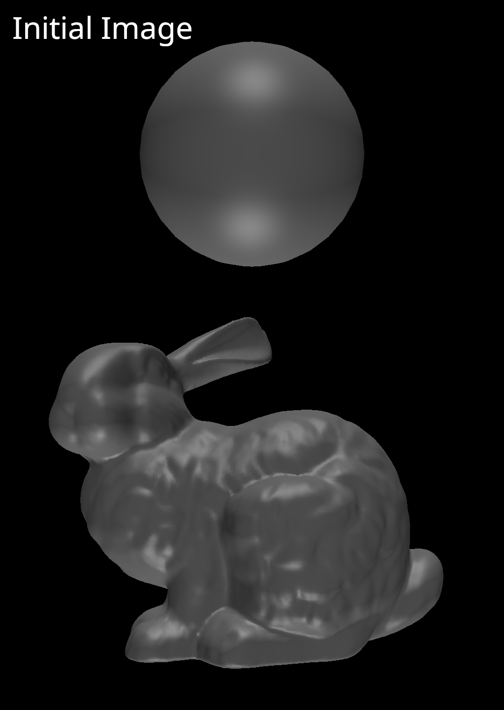
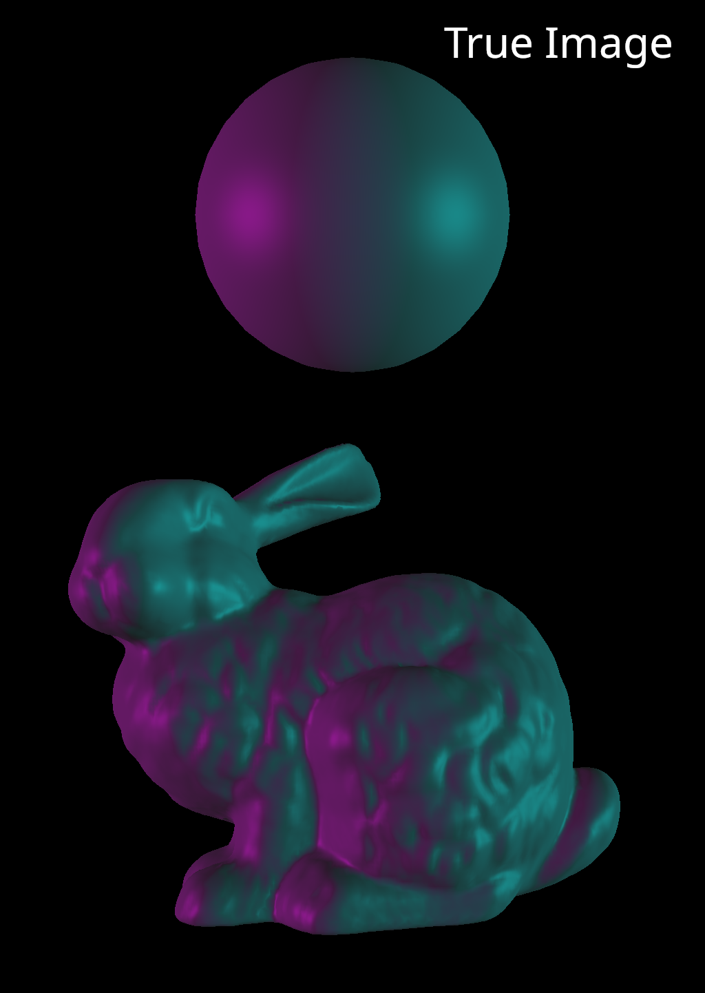
Here is a figure showing true and initial images for two different meshes illuminated by two directional lights. The true lighting configuration uses a teal and a purple light aimed at the left and the right sides of the meshes. The initial lighting configuration uses white lights aimed at the top and the bottom of the meshes. The optimization process should recover the true color and position of the lights.
Here is a video showing the optimization process for the spherical mesh. It’s easy to see how the lights change on such a simple geometric surface.
That worked beautifully! Now let’s try the bunny, which has a much more complicated surface.
Looks great! Our reverse-mode AD is working, and we can perform gradient descent optimzation on light parameters.
Optimizing Albedo
Let’s now try to optimize albedo paramters.
This is a very natural extension of what we have just done.
The shader grad() kernel backpropagates gradients to the albedo G-buffer already.
To optimize for albedo parameters, we need simply backpropagate our gradients one more step through the albedo interpolator and update our per-vertex albedo values.
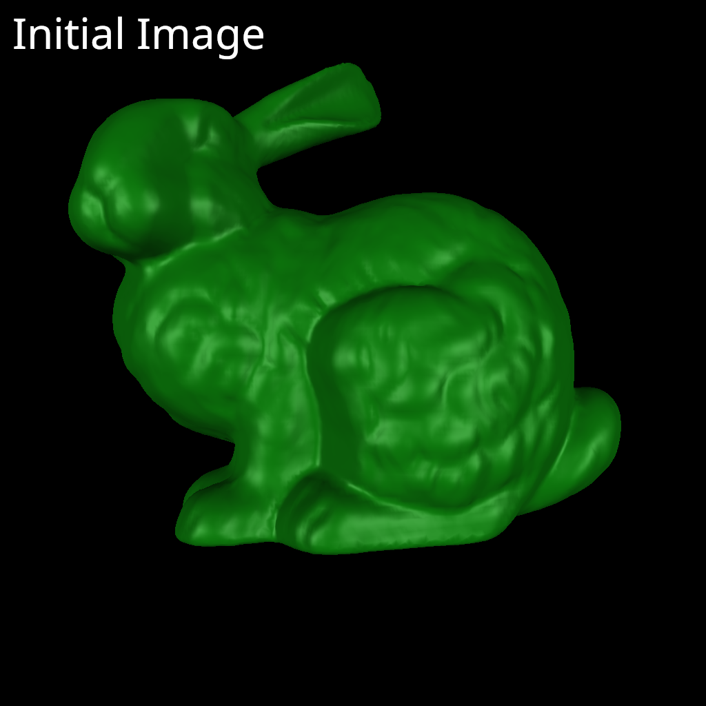
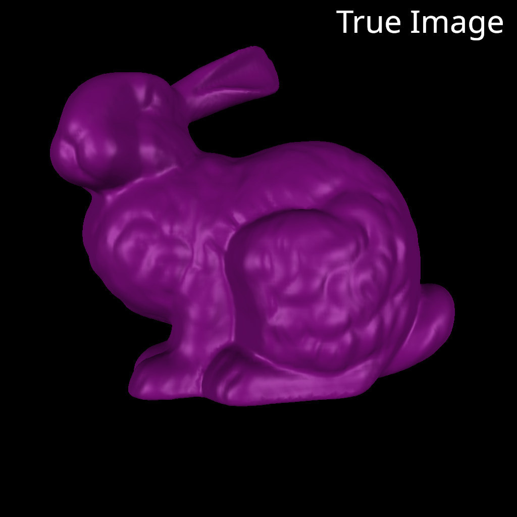
Let’s set up an experiment where the ground truth albedos are purple, and our initial albedos are green. Albedo is defined per-vertex, so we we will actually only be able to learn the albedos of vertices that are visible from our camera. We could add additional cameras if we wanted to learn parameters for the entire mesh. In this example, we use white lights.
Here is a video showing the optimization process for the bunny mesh.
Notice that certain vertex albedos converge more quickly to the true color than others. The rate of convergence depends on the magnitude of the gradients at each albedo parameter, which depends on the contribution of each parameter to the rendered image. Vertex albedos associated with triangles that cover many pixels in the image recieve larger gradients and converge faster.
Coding Challenge 6
The coding challenge for this post is to implement your own version of the experiments described above. Again, this mostly involves making use of the existing rendering pipeline combined with the AD functionality of Taichi. As always, we will provide some additional discussion about our implementation below. You can also go look at the project codebase to see exactly how our implementation works.
Implementation
Optimizing Lighting
For these optimization experiment, we need a scalar loss function and a method that updates parameters.
Let’s start with the loss.
We will use a simple mean squared error.
This class is quite simple.
We need an image buffer field, a field to store the reference ground truth image that we will compare against, and a loss field.
Finally, we need a kernel to compute the loss.
We also have forward() and backward() methods to keep things organized.
@ti.data_oriented
class ImageMeanSquaredError:
    def __init__(
        self,
        image_buffer: ti.Vector.field,
    ):

        self.image_buffer = image_buffer

        image_shape = image_buffer.shape
        self.n_pixels = float(image_shape[0] * image_shape[1])

        self.reference_buffer = ti.Vector.field(
            n=image_buffer.n, dtype=float, shape=image_shape
        )
        self.loss = ti.field(float, shape=(), needs_grad=True)

    def forward(self):
        self.clear()
        self.compute_loss()

    def clear(self):
        self.loss.fill(0)
        self.loss.grad.fill(0)

    def backward(self):
        self.loss.grad.fill(1.0)
        self.compute_loss.grad()

    def set_reference_image(self, reference_image: np.array):
        self.reference_buffer.from_numpy(reference_image)

    @ti.kernel
    def compute_loss(self):
        for i, j in self.image_buffer:
            pass # Your code here
After adding the loss function to our pipeline and updating the forward() and backwards() methods to include the loss, we just need an update method.
For the light optimization experiment, the pipeline update method just calls update on the light array with a learning rate parameter.
def update(self):
    self.light_array.update(self.lr)
The light array update method updates the light color and direction fields according to their gradient fields and the learning rate. We also make sure that the light direction remains a unit vector using normalization.
@ti.kernel
def update(self, lr: float):
    for i in range(self.n_lights):
        self.light_colors[i] = self.light_colors[i] - lr * self.light_colors.grad[i]
        self.light_directions[i] = tm.normalize(
            self.light_directions[i] - lr * self.light_directions.grad[i]
        )
    self.light_colors.grad.fill(0)
    self.light_directions.grad.fill(0)
This is the simplest possible form of gradient descent optimization. Many optimizers will incorporate momentum terms and other more sophisticated features. If you are interested, you could also try to write a more complex optimizer.
The final step in the optimization experiment is to run the training loop.
This involves iteratively calling forward, backward and update.
We will leave those implementation details in the codebase in case you get stuck.
Optimizing Albedos
To optimize albedo values, we simply need to extend our backwards and update methods.
The gradients must reach the albedo field through the albedo interpolator, and the albedo values must be updated.
In your explorations, try to make sure you understand which data fields are recieving gradients when you call .grad() on kernels.
In PyTorch and other ML frameworks, this accounting is typically hidden from the user using gradient tape.
Taichi also has functionality for gradient tape, but managing backpropagation manually is a very good way of checking your understanding and debugging if things go wrong.
Conclusion
In this lesson we performed our first piece of inverse rendering! We optimized light and albedo parameters using gradient descent. In the next lessons we will continue to step backwards through the pipeline and perform similar optimization experiments for camera, and mesh vertex parameters. Soon, we will re-encounter the discontinuity problem, and this time we will implement some solutions.