Welcome back! In the last lesson, we learned light and albedo scene parameters from image supervision using a differentiable rendering pipeline and gradient descent optimization. For those experiments, we found that we did not encounter any issues with boundary discontinuities. That will not be the case going forwards. In this lesson, we will once again encounter the discontinuity problem. We will then review the different approaches that have been proposed to solve the problem in a rasterization pipeline, and select a couple to implement in our codebase.

Contents

Visualizing The Discontinuity Problem

A couple of lessons ago, we created Jacobian images that showed the partial derivative of a rendered image with respect to light direction parameters. Let’s now create a Jacobian image with respect to a mesh translation parameter. In other words, our Jacobian image will show how each pixel of the image changes as a mesh is translated in world space. We will again use a simple rendering of a phong shaded sphere with a white directional light for our example.

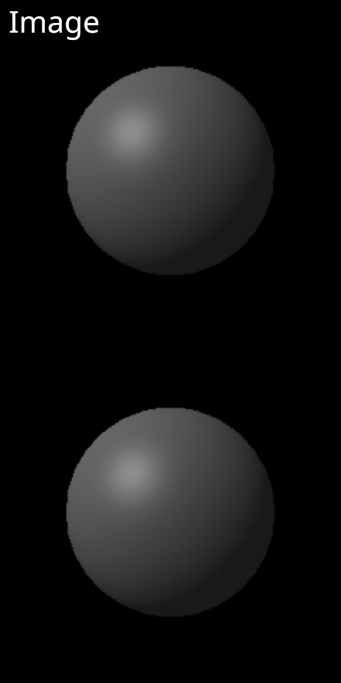
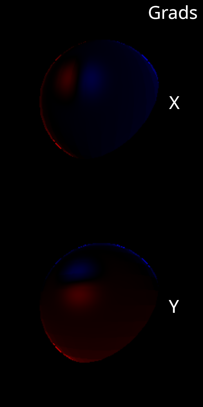
A sphere rendered with Blinn-Phong shading and a single white directional light. The gradient images show the partial derivative of each pixel with respect to the x and y components of a mesh translation

There are aspects of this Jacobian image that look correct. The area around the specular highlight makes sense. We can also see the largest values are near the silhouette of the sphere. This makes sense because the surface is nearly orthogonal to the camera view direction in this area. Therefore, small changes in the sphere position can lead to very large changes in the barycentric buffer coordinates that propagate through to the final rendered image.

However, there are other aspects of the image that do not make sense. For example, the bottom right portion of the sphere is not lit by the directional light and therefore, only has non-zero shading due to the ambient component. The gradient at the sillhouette for this part of the sphere is zero. This is obviously not correct as translating the sphere will move the boundary, which will cause some pixels to change in value. As you probably guessed, this is the discontinuity problem rearing it’s ugly head again.

We can make this issue crystal clear by simplifying our shader so that our rendered image is a mask with no variation due to lighting. We are going to call this a silhouette image. The use of silhouette images is very common in inverse rendering experiments because the only non-zero gradients in this type of image come at the silhouette boundaries. Therefore, if your boundary gradients aren’t working properly, it will be very obvious. Let’s now visualize a silhouette image and it’s Jacobian image with respect to mesh translation.

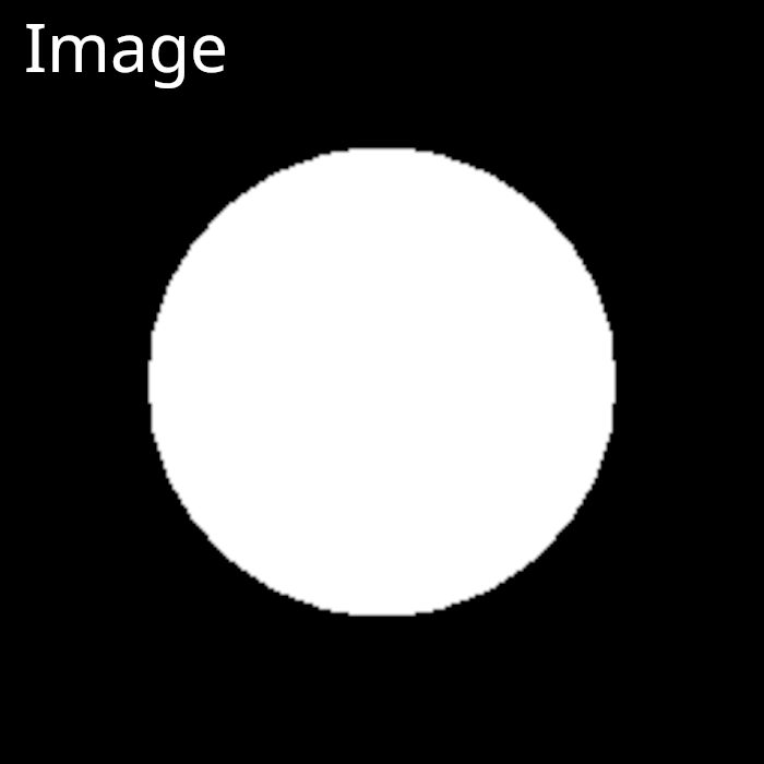
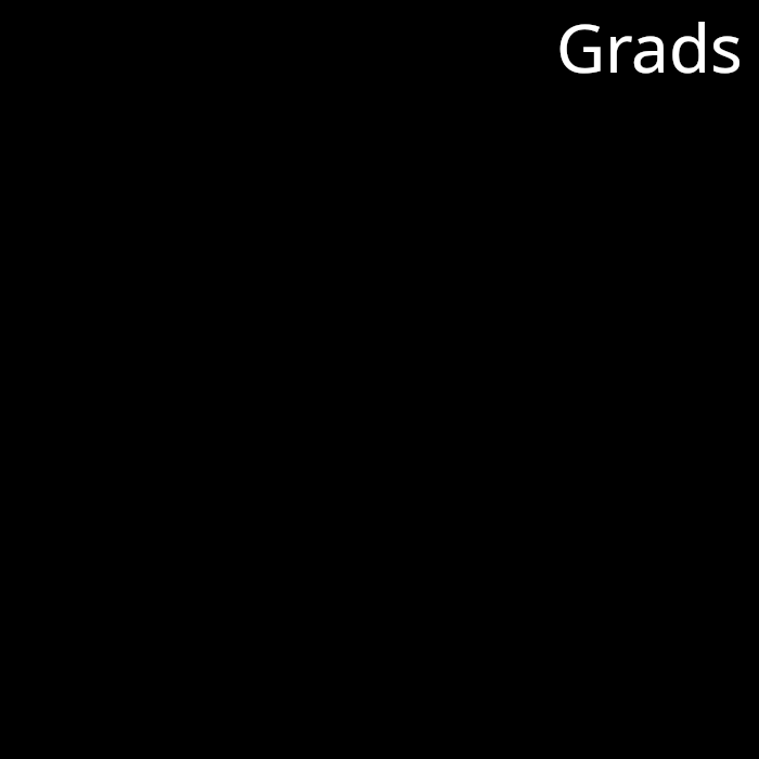
A sphere rendered with silhouette shading. The gradient images with respect to the x and y components of a mesh translation are zero.

Now it is much easier to see that there is something wrong with our boundary gradients. The gradients for this example are zero everywhere in the image, just like we saw in our 2D triangle rasterizer at the start of the course. Therefore, we will be completely unable to, for example, learn the position of this sphere using gradient descent, as we did for light and albedo parameters in the previous lesson. It is now time to dig into this problem and find a solution or two that we can implement in our codebase.

Solving The Discontinuity Problem

Overall, the most popular solution to the discontinuity problem is to take the hard step functions that we find at silhouette boundaries and make them soft somehow. In making the boundaries soft, we must also ensure that the pixel values relate continuously to the vertex positions, thereby enabling backpropagation. There have been many different variations and implementations of this high level solution. The trick is in doing it well and efficiently.

It is also worth noting that there is a parallel line of work in the ray tracing space. The discontinuity problem appears also appears there in a more complicated form. Ray tracing formulates the calculation of pixel color as an integral. Therefore, differentiable ray tracing involves taking the partial derivative of an integral. The state-of-the-art work in this space involves methods to re-parameterize integrals so as to admit differentiation with respect to discontinuous parameters. We won’t be reviewing this work here, however. Perhaps in a future course.

Older Work

One of the first general purpose differentiable rasterization approaches was OpenDR, published in 2014. OpenDR used a filtering approach on the final rendering image to compute gradients (with consideration for which pixels represent silhouette boundaries). The approach is actually quite similar to taking finite differences. The downsides of this approach include a lack of support for differentiation with respect to textures, and incorrect gradients in certain scenarios. For example, shading details like specular highlights are treated as if they are part of the mesh surface and move with the surface of the mesh. If we rotate a rendered sphere about it’s origin, the specular highlights will actually slide along the mesh surface as the sphere rotates, remaining stationary in the image.

Later publications Neural Mesh Renderer and Soft-Ras perform rasterization with different varieties of blur and transparency integrated into the rasterization process. Both of these methods do not scale well with mesh complexity, and can become very computationally expensive for large meshes. DIB-R is a newer method proposed by Nvidia researchers that uses an additional alpha channel to approximate silhouette boundary gradients. However, this approach requires that an alpha mask be available for reference images, and is not able to produce correct gradients for sillhouetes against visible geometry (as opposed to silhouettes against a background color/image).

More recently, two approaches have been proposed that address many of the limitations of older approaches. These approaches are now core algorithms in 3D machine learning packages like PyTorch3D, Kaolin, and Tensorflow Graphics. Our focus going forwards will be to understand and implement these two approaches.

Nvidia DiffRast (NVDR)

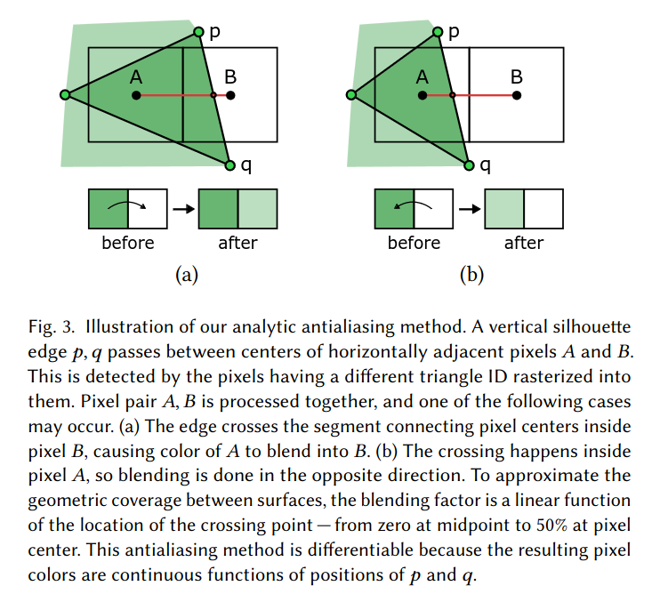
In 2020, Nvidia researchers published an approach (NVDR) based on an anti-aliasing operation. The approach makes use of deferred shading (which enables support for arbitrary shading approaches), and scales well with mesh complexity (which greatly improves the performance of inverse rendering). They also released tightly optimized, modular CUDA kernels, which enabled widespread adoption of their work. Their core idea was to solve the discontinuity problem by blurring pairs of pixels that span either side of a silhouette boundary. The amount and direction of blurring is dependent on where the silhouette edge passes between the pixel pair. Thus, the operation, which is placed at the very end of a rasterization pipeline, allows sillhouette boundary gradients to flow from the final image, to the clip coordinates of the triangle mesh vertices.

The antialiasing operation proposed in NVDR. Figure taken from Laine et al.

Rasterize-Then-Splat (RTS)

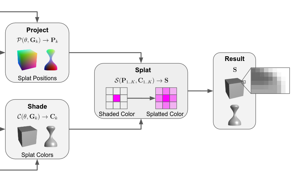
In 2021, Google researchers published an approach (RTS) based on a splatting operation. This approach is competitive with NVDR in terms of performance, and also solves a notable limitation of NVDR. NVDR has a tendency to miss gradients at some silhouette boundary pixels when meshes are very finely tesselated, or when using low image resolution. We will discuss this issue more in a future lesson. The RTS splatting operation takes pixel colors and “splats” them in a 3x3 pixel neighborhood using a small Gaussian kernel. Thus, the hard boundaries are made soft through mild blurring. The gradients of the splatted image are then backpropagated through specialized G-buffers to the geometry scene parameters without passing through the rasterizer directly.

The splatting operation in the RTS pipeline. Cropped figure taken from Cole et al.

Coding Challenge 7

The challenge for this lesson is to visualize the discontinuity problem for yourself in a 3D rasterization pipeline. In previous lessons we learned about the Taichi AD system and used it to create Jacobian images and learn parameters. For this experiment, we need simply extend our AD experiments by one more step and attempt to backpropagate gradients through the rasterization stage of our pipeline. You can also try optimizing parameters like mesh vertices or camera position and orientation. Just don’t expect it to work yet.

Conclusion

In this lesson, we re-encountered the discontinuity problem and reviewed, at a high level, the approaches that have been proposed to solve it. In particular, we identified two approaches as state-of-the-art in differentiable triangle rasterization. In future lessons, we will cover NVDR and RTS in much greater detail and implement them within our codebase.