1) The Discontinuity Problem
Welcome back! Now that the preliminaries are dealt with, we are ready to dive into the world of inverse rendering.
In this lesson, we are going to write a 2D rasterizer that renders a single triangle. In future lessons, we will gradually be developing a proper 3D rendering engine. We are using this simple example to explore the discontinuity problem. This is a core problem for differentiable rendering algorithms, and one of the reasons why special algorithms are required. This will also provide a good opportunity to familiarize ourselves with some basic features of Taichi.
Contents
Discussion
This structure of this lesson also resembles the overall structure of the course. We will first implement the forward pass, in which scene parameters are turned into a rendered image. Afterwards, we will implement the backward pass, in which gradients are backpropagated from the output image to the scene parameters.
Forward
The forward process for our example turns a 2D triangle defined by 3 vertices \(\in \mathbb{R}^2\) into an image buffer. Let’s start by defining a triangle in Taichi and setting some initial values.
import taichi as ti
import taichi.math as tm

ti.init(arch=ti.gpu)

triangle = ti.Vector.field(dtype=ti.f32, n=2, shape=(3), needs_grad=True)
triangle[0] = tm.vec2(10.1, 10.2)
triangle[1] = tm.vec2(90.3, 10.4)
triangle[2] = tm.vec2(50.5, 50.6)
After the imports, we call ti.init.
As described in the Taichi docs, this is required and is used to specify the backend that will execute our compiled code, along with other compilation options.
Here, we are asking for a GPU backend, but it will fallback to CPU if no GPU is available.
Next, we are defining a field data container for our 2D triangle.
Taichi fields are global, mutable data containers and we will be using them extensively in our codebase.
In this case, we are using a 2D vector field, which means that each of the 3 elements in our field is a 2D vector.
We also indicate the dtype of our field (32 bit floating point) and specify that the field needs gradients.
We will have more to say about gradients when we look at the backward pass.
So far so good. Let’s try defining an image buffer now. We will be generating a grayscale image, so no need for a vector field here. We will also use a buffer size of 100x100 pixels.
image = ti.field(dtype=ti.f32, shape=(100, 100), needs_grad=True)
Now that we have our data fields, we need to write some code to run the forward pass.
We could write it using pure python, but we want to access the power of Taichi.
To write Taichi code, we must use some special decorators.
@ti.kernel is used to define a kernel function.
Much like in CUDA, kernels can be called from the host (python), but they cannot be called from other kernels or device functions.
@ti.func is used to define a device function.
Device functions cannot be called from the host, but they can be called from kernels or other device functions.
Taichi and python look alike, but are not identical. It’s important to remember that code within a kernel or device function will be compiled and executed by Taichi.
Let’s start by writing a render kernel.
@ti.kernel
def render():
    for pixel in ti.grouped(image):
        if is_pixel_in_triangle(pixel):
            image[*pixel] = 1.0
        else:
            image[*pixel] = 0.0
This kernel iterates over each pixel in the image.
For each pixel, it calls a device functionis_pixel_in_triangle which returns true if the pixel is within the bounds of the triangle.
If the pixel is in the triangle, the pixel value is set to 1.
If the pixel is not in the triangle, the pixel value is set to 0.
This may look like a regular python for-loop, which we know can be quite slow.
However, this loop is lightning fast thanks to one of the most powerful features of Taichi.
Any for-loop in the outermost scope of a Taichi kernel will be automatically parallelized unless it is specifically directed to execute serially.
This means that each pixel is processed in parallel (at the same time) and not in sequence, as they would be in a python for-loop.
Furthermore, if we are running this code on a machine with a GPU, Taichi will compile the kernel and run it on the GPU.
Pretty awesome, right?!
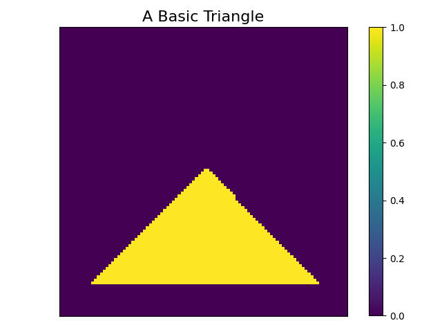
Once we have a working render kernel, we can generate images of our triangle that looks something like this.
We will use the Taichi visualization tools in future lessons.
For now, we will simply convert our Taichi image field to a numpy array with image.to_numpy() and visualize it with matplotlib.
Before going backward, we will quickly write a simple kernel to compute a scalar loss. For the sake of simplicity, our loss just computes a sum over all the image pixels. Minimizing this loss would correspond to shrinking the triangle so that it occupies fewer pixels in the image.
loss = ti.field(dtype=ti.f32, shape=(), needs_grad=True)

@ti.kernel
def compute_loss():
    for pixel in ti.grouped(image):
        loss[None] += image[*pixel]
We can render an image and compute the loss by running our Taichi kernels in sequence. The loss for this triangle is 1610.
render()
compute_loss()
print("Loss = ", loss[None])

"""
Loss = 1610.0
"""
Backward
Now we’re ready to go backward using the automatic differentiation (AD) features of Taichi. If you are completely unfamiliar with AD, this is probably a good time to do some additional reading. Taichi has good documentation describing it’s AD support. There are also some good youtube videos that provide a gentler introduction to the topic. We will exclusively be using reverse-mode AD in this project, but it’s very useful to understand forward-mode AD and how all of these operations relate to Jacobian matrices, vector-Jacobian products, and Jacobian-vector products. We will also discuss these points in detail in a future lesson, so don’t feel like you need to be an AD master just yet.
In this project, we will always call our gradient kernels manually to make sure that it is clear what is happening. Calling a gradient kernel will back-propagate the gradients from the output fields of the kernel, to the input fields of the kernel. Taichi AD is different from ML libraries like Jax, Tensorflow and PyTorch because Taichi fields are mutable. Therefore, if you are used to AD in ML libraries, I strongly recommend that you take a peek at the docs to understand the differences.
Returning to our code.
Let’s now try to backpropagate gradients from our loss to the triangle vertices.
In the context of inverse rendering, this gradient will provide the information required to update the triangle vertex parameters.
To begin, we can call the gradient kernel of our compute_loss kernel to backpropagate gradients from the loss field to the image field.
Taichi will automatically compile gradient kernels so we don’t need to write any custom code!
In Taichi, we must first seed our gradient field, which we do by setting it to 1.
loss.grad[None] = 1.0
compute_loss.grad()
Now let’s visualize the gradient of the image field (accessed with image.grad) to see what the result of that operation was.
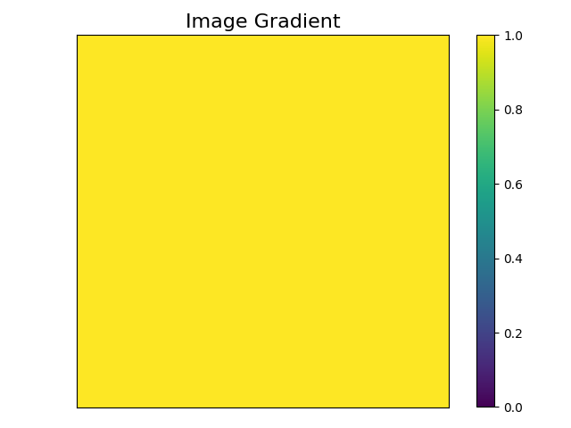
This is exactly what we would expect to see.
The partial derivative of the loss with respect to any pixel in the image is 1.
Now, let’s call render.grad() to back-propagate the image gradients to the triangle vertices.
render.grad()
print(Triangle Grad)
print(triangle.grad.to_numpy())

"""
Triangle Grad
[[0. 0.]
 [0. 0.]
 [0. 0.]]
"""
Now, it looks we have a problem… The resulting gradient vector is 0 for all of the triangle vertices. If our gradients are 0, we won’t be able to update/learn the triangle parameters. But how could our gradients be 0!? We know that the image loss must change if the triangle vertices change, right? Maybe this is a bug in Taichi. Let’s try computing a finite difference by perturbing one of the triangle vertices and re-computing the loss.
loss.fill(0.0)
triangle[2].y += 1e-5
render()
compute_loss()
print("Perturbed Loss = ", loss[None])

"""
Perturbed Loss = 1610.0
"""
The loss is exactly the same! Something is definitely going on here. Let’s investigate further by plotting the loss as a function of perturbation size.
loss_sequence = []
for i in range(10000):
    loss.fill(0.0)
    triangle[2].y += 1e-5
    render()
    compute_loss()
    loss_sequence.append(loss[None])
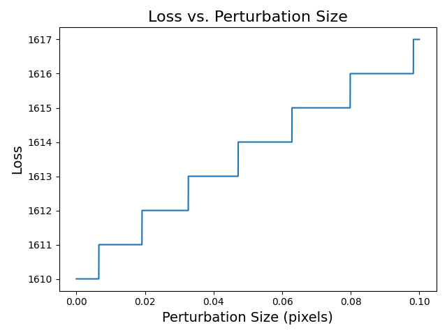
Things are starting to become a bit clearer. We were (of course) correct in thinking that the loss is a function of the triangle vertex coordinates. However, the loss doesn’t change in a continuous way. Only once a triangle vertex changes enough to cause one or more pixels to flip from being inside the triangle to outside the triangle (or vice versa) will the loss function change in value.
This is what we call the discontinuity problem, and it is indeed a problem if we want to perform inverse rendering. The derivative of our loss function with respect to our geometry parameters is 0 almost everywhere and does not provide any useful information for how to update our triangle geometry. At the same time, if we squint our eyes, we can see that there is clearly a positive relationship between the loss and the size of the perturbation in our experiment. In fact, the only reason this problem arises in the first place is because we are discretizing our image by sampling it at pixel coordinates. The rendering process is naturally continuous if we think of the image as a continuous domain. Unfortunately, we must discretize the image in order to perform rendering using a digital computer. What we need, is some way of recovering the gradient information so that we know how to update our triangle parameters. This is exactly what differentiable rasterization approaches aim to do, and what we will do in future lessons, but not today. For now, I recommend that you spend a few minutes thinking about how this problem might be solved and what challenges might be involved in solving it.
Coding Challenge 1
Now it’s your turn to write some Taichi code. The challenge for this lesson is to replicate our experiment demonstrating the discontinuity problem. All that is left to complete our 2D triangle rasterizer implementation is a device function that tells us if a pixel is inside of the triangle. Something that looks like this:
@ti.func
def is_pixel_in_triangle(pixel: tm.vec2) -> bool:
    pass # Your code here
If you are unsure of where to start with this challenge, we highly recommend that you read The Barycentric Conspiracy blog post by Fabian “ryg” Giesen. Throughout this project, we will try to avoid duplicating educational content on topics for which excellent educational content already exists. Whenever appropriate, we will direct you to these sources so that the content in this project can focus on special aspects of differentiable triangle rasterization.
As always, you can also refer to the project codebase to see a working solution for this challenge.
Conclusion
In this lesson, we used a simple 2D triangle rasterizer to explore the discontinuity problem. We saw that this problem prevents us from learning and updating triangle vertex parameters. We also wrote our first code in Taichi and brushed up on the basics of triangle rasterization and automatic differentiation. In the next lesson we will leave flatland and begin building a full 3D rasterization pipeline, starting with camera models.