2) Learnable Camera Models
Welcome back! In this lesson, we will be taking the first steps towards building a differentiable 3D renderer.
All rendering algorithms need some way to define the properties of a camera that will capture a rendered image. We will implement both orthographic, and perspective (or pinhole) camera models, as is typical for a rasterization approach. We will also discuss some special considerations associated with learnable camera models. In doing so, we will learn a bit about group theory, and the importance of continuous data representations in machine learning.
Contents
Discussion
The Rasterization Pipeline
Before we dive into camera models, it’s helpful to review the rasterization pipeline and how camera models fit into it. At a high level, rasterization works by mapping triangles that are initially represented in what can be called world space into a different coordinate system that can be called screen space. Be warned that the specific terminology used for these coordinate systems can vary. Once triangle vertices are represented in screen space, the triangles are drawn on the image buffer, as we saw in the previous lesson. The mapping from world space to screen space is performed such that the triangle representation in screen space reflects how the triangles appear from the point of view of a camera. Therefore, the camera model and the parameters of the camera are essential in defining this mapping.

The mapping from world space to screen space can be broken down into different stages.
The first stage is a mapping from world space to view space and is defined by a view matrix.
The view matrix encodes information about the position and orientation (rotation) of a camera.
The second stage is a mapping from view space to clip space and is defined by a projection matrix.
the projection matrix encodes information about the camera model (orthographic or perspective) as well as additional camera parameters like field of view.
The view and projection matrices are both 4x4 matrices that use homogeneous coordinates.
This approach to implementing camera transformations is consequential in both positive and negative ways. On one hand, it is part of what allows rasterization approaches to be so fast and computationally efficient compared to other rendering approaches like ray tracing. Once geometry is represented in screen space, it is much easier to compute which geometric elements intersect the view direction associated with each image pixel. On the other hand, it limits the type of camera model that can be used. Orthographic and pinhole perspective cameras both fit well into this approach because they are rectilinear. Straight lines (such as triangle edges) in world space also appear straight in images that are taken with rectilinear cameras. Camera models that have non-pinhole aperatures and realistic lens systems with distortion cannot be easily implemented using this approach. Therefore, effects like depth of field, lens distortion, and other phenomenon observed in photography will not work, or must be approximated somehow, using rasterization. This will not deter us. Orthographic and pinhole camera models are still very useful, but, we must keep their limitations in mind.
In developing our 3D rasterizer, we will need to implement all of these transformations. If these ideas are new to you, or you just want a quick refresher, here are a few additional resources that describe the different coordinate systems and the transformations between them. Learn OpenGL has a good article that provides a high level overview. Song Ho has a nice article that covers the transformation matrices in detail. The tiny renderer project also has good content on this topic. Finally, if you are completely new to this space, you may need to spend some time learning about homogeneous coordinate systems. Here is a good lecture that will help you understand the math that is used throughout this transformation process.
Considerations for Learnability
Now that we are up to speed on the details of how the camera parameters enter the rasterization pipeline, we are ready to think about how to implement our camera models. Once we start performing inverse rendering, we will be trying to learn camera parameters using gradient descent. Therefore, we should take some time here to think of any special considerations that may apply to the problem of implementing learnable camera models. We are going to focus on the view matrix, which encodes the position and orientation of our camera. Some of the considerations we discuss are also applicable to the projection matrix, which happens to be simpler. In our codebase, we only implement cameras with learnable position and rotation, although it is certainly possible to learn other camera parameters like field of view.
We know that the camera view matrix is a homogeneous 4x4 matrix that represents the composition of a translation and a rotation transformation. Let’s start by considering an inverse rendering approach in which we represent our camera position and orientation with a 4x4 view matrix directly and learn the parameters of the matrix through gradient descent. Take a moment and see if you can think of any issues that might arise with this approach.
An important question we must ask ourselves here is: “are there any 4x4 matrices which do not represent valid view matrices?”. The answer is, of course, yes! Take another moment and see if you can think of one or two. This turns out to be a serious issue for the proposal to represent and learn camera parameters using the view matrix directly. The learning algorithm knows nothing about what is or is not a valid view matrix and may produce invalid matrices in order to minimize the loss. We could just hope that whatever matrix is learned turns out to be valid, but this does not seem like a sound approach. It would be better to use a constrained representation of our cameras to ensure that invalid camera matrices are never encountered. Implementing constraints of this type is quite common in machine learning and statistics. For example, when training a model whose output is intended to be a probability value, it is good practice to use a logistic or softmax function to ensure that the output is always a valid probability between 0 and 1.
Let’s consider a different proposition then. What if we were to represent the position and orientation of our camera using a 3D vector defining the camera position and a second 3D vector defining the camera orientation in terms of three Euler angles (yaw, pitch and roll). We could then construct our view matrix from this representation before applying the matrix in our rasterization pipeline. This would ensure that the view matrix we construct is always valid. Take another moment for reflection. Can you think of any issues that might arise with this approach?
This time, the issue is more subtle. The method of representing camera position using a 3D vector seems sound, but the rotational component requires some additional thought. If you are familiar with the mathematics of rotation in 3D, you may have heard of the phenomenon of gimbal lock that can occur when using Euler angles. Do you think that this phenomenon could cause issues in the process of learning camera parameters? Maybe you have heard of quaternions which can also be used to represent rotations in 3D. Should we instead use a quaternion representation for the rotational component of our camera? What are the important properties that we should consider for when selecting a learnable rotation representation? These are not easy questions and they require a systematic investigation. Thankfully, there is an excellent paper on this exact topic whose results and conclusions we will now review.
Learning on \(\mathrm{SO}(3)\)
The 2019 paper that we will be reviewing here, and using as the basis for our implementation of learnable camera rotation, is On the Continuity of Rotation Representations in Neural Networks by Zhou and Barnes et al. This paper tackles the issue of how to select appropriate representations for learnable rotations.
To start, it’s helpful to understand that the set of rotations in 3D dimensions has a special structure. The set, along with the operation of matrix composition, forms a mathematical group. Furthermore, the set is also a differentiable manifold. Groups that are also differentiable manifolds are called Lie groups and they provide a natural model for the concept of continuous symmetries.
Let’s now consider the symmetry group of a sphere in 3 dimensions. This group, denoted \(\mathrm{O}(3)\), is known as the orthogonal group. It is the set of all linear transformations under which a 3D sphere is invariant. In other words, it consists of all linear transformations that map a 3D sphere centered at the origin back into the exact same 3D sphere. The special orthogonal group, denoted \(\mathrm{SO}(3)\) is a sub-group of \(\mathrm{O}(3)\). It includes only the elements of \(\mathrm{O}(3)\) with determinant equal to 1 (thereby excluding transformations that involve reflection). \(\mathrm{SO}(3)\) is, in other words, a group which contains all rotation transformations in 3D, and it is the object of our interest today. It is not necessary to be an expert in group theory for our purposes, but it is helpful to understand a bit of the background because the paper that we are reviewing frequently uses notation and terminology from group theory.
Following Zhou and Barnes, let’s now introduce the concept of an original space \(X\), and a representation space \(R\). In our problem, the original space corresponds to a rotation matrix, and the representation space corresponds to some representation of the rotation matrix (e.g. a 3D vector of Euler angles). The idea here is that our learnable parameters will live in the representation space and will be mapped into the original space for use in our rendering algorithm. To be a valid representation, there must be a mapping from the representation space to the original space \(f: R \rightarrow X\) , and a mapping from the original space to the representation space \(g: X \rightarrow R\) such that \(\forall x \in X, f \circ g(x) = x\). In other words, \(f\) is a left inverse of \(g\).
Next, the paper introduces the concept of a continuous representation. A representation is continuous if \(g\) is continuous. The core claim of the paper is that continuous representations are important because the process of learning through gradient descent is a gradual and path-dependent process. Intuitively, you can think of a discontinuous representation as one in which there is a gap in the representation space over which the learning process cannot jump. The presence of these gaps can block the learning process and prevent it from converging to an optimal result.
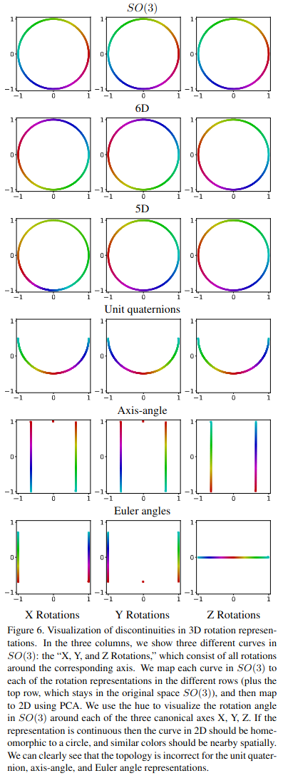
With this new theory in hand, let us return to our quest to find a representation for the rotational component of our camera. We now know that we are looking for a continous representation of \(\mathrm{SO}(3)\). We had previously considered Euler angles and quaternions. Are either of these representations continuous? It turns out that the answer is no! In fact, Zhou and Barnes et al. show that for 3D rotations, all Euclidean representations of 4 or fewer dimensions are discontinuous. They go on to derive 5 and 6 dimensional representations that are continuous. Here is an excellent figure that visually summarizes their result.
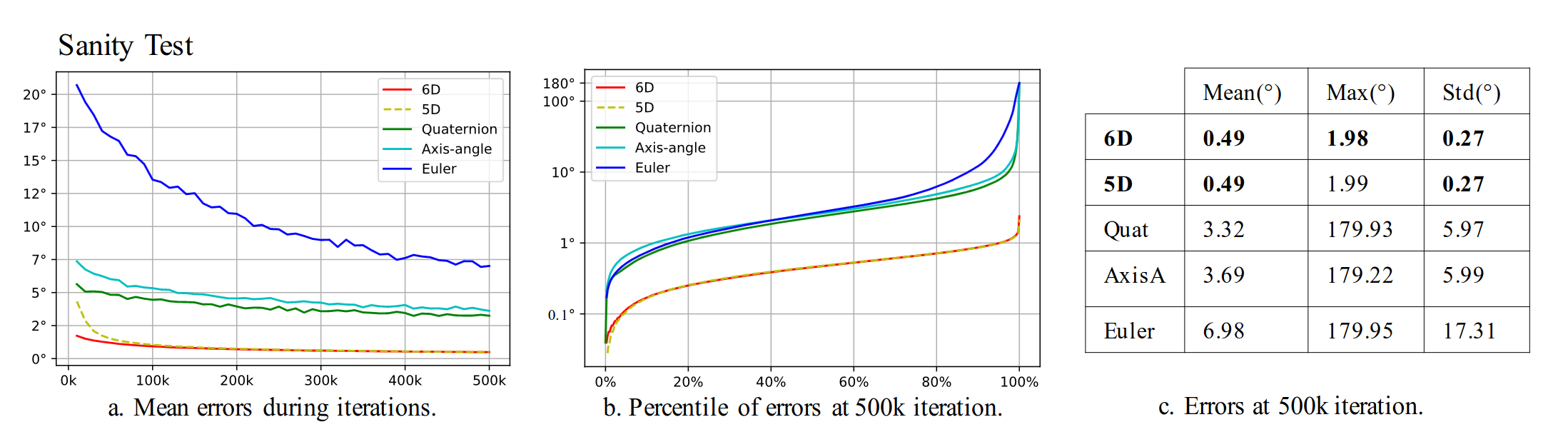
You may be asking yourself if this actually matters in practice. Is using a discontinous representation like quaternions or Euler angles really going to effect the process of learning a rotation? The anwer will depend on the details of the optimization problem. Perhaps the rotation that is being optimized can be initialized very close to the true solution, such that discontinuities in the selected representation space are never encountered. Or, perhaps the rotation optimization can be further constrained to a single dimension. In these scenarios, you could probably get away with using an Euler angle representation, provided you are mindful of the discontinuous nature of that representation. For general rotation optimization problems, discontinuous representations can absolutely cause performance issues. The authors performed a series of experiments to validate their work, and all of their experiments showed a clear difference in performance for general rotation estimation tasks. Here is a snapshot of their sanity check experiment results. Look at the difference in maximum errors between their continuous 5 and 6D representations and other approaches. Using a continuous representation can mean the difference between 180 degrees and 2 degrees of rotational error!
Before moving on from this paper, let’s review their surprisingly simple 6D rotation representation of \(\mathrm{SO}(3)\) beginning with the mapping \(g: X \rightarrow R\). Equations 15 and 16 from supplemental section B provide everything we need to know. First, we will note that a rotation in 3D can be fully and uniquely described using 3D basis vectors \(\{\hat{x}, \hat{y}, \hat{z}\}\) that, together, make a 9D representation. Next, we will note that one of these vectors is redundant. Coordinate systems follow a left or right hand convention and no rotation is capable of flipping that convention. Therefore, we can create a 6D representation with any two of the basis vectors, such as \(\{\hat{x}, \hat{y}\}\). Wonderfully simple!
Now let’s look at how to implement \(f: R \rightarrow X\) with \(R = \mathbb{R}^6\). We begin by taking the first 3 elements of \(r \in R\), treat them as a single vector \(\in \mathbb{R}^3\), and normalize the vector to create a unit vector that we will call \(\hat{x}\). Next, we take the second 3 elements of \(r\), treat them as a single vector \(\in \mathbb{R}^3\), project the vector onto a plane such that it is orthogonal to \(\hat{x}\), and then normalize it to create a unit vector that we will call \(\hat{y}\). Finally, we take a cross product \(\hat{z} = \hat{x} \times \hat{y}\). We have recovered a basis \(\{ \hat{x}, \hat{y}, \hat{z}\}\) that defines a rotation in 3D. Notice that this is a valid representation, because the property \(\forall x \in X, f \circ g(x) = x\) holds true. It is also a continuous representation because \(g\) is continuous. This is all we will say about this paper here, but I encourage you to read it in detail as the authors do an great job of presenting and explaining their work.
Coding Challenge 2
The coding challenge for this lesson is to implement learnable perspective and orthographic camera models using the 6D rotation representation proposed by Zhou and Barnes et al.
Going forwards, we will accompany the coding challenges with some additional details on how it is implemented in our codebase (without giving everything away). As always, you can go look at the codebase for working implementations of this challenge if you want. If you would like, you can use these details as a skeleton for your solution to the challenge, or you can just do your own thing. Please do not take our implementation as the correct answer to these challenges, but rather as a correct answer. It’s very possible that you will come up with some clever solution that is better than ours. If you do, don’t hesitate to let us know!
Implementation
In the project codebase, Taichi’s @data_oriented class decorator is used quite extensively to keep things organized.
This decorator allows you to create a python class with Taichi kernels and device functions as member functions.
The kernels and device functions can access any Taichi fields that are members of the class.
Within the codebase there is a class for rigid transforms.
This class implements a learnable continuous representation of the special Euclidean group \(\mathrm{SE}(3)\) that includes both rotation and translation transformations.
The class has member variables for a 3D position parameter, a 6D rotation parameter, and a \(4 \times 4\) transformation matrix in homogeneous coordinates.
The class has a compute_matrix kernel which implements the logic related to the function \(f: R \rightarrow X\).
The class also has python methods forward, backward, and clear for convienence.
@ti.data_oriented
class RigidTransform:
 def __init__(self):
        self.position_param = ti.Vector.field(n=3, dtype=float, shape=(), needs_grad=True)
        self.rotation_param = ti.Vector.field(n=3, dtype=float, shape=(2), needs_grad=True)
        self.matrix = ti.Matrix.field(4,4, float, shape=(), needs_grad=True)

        # Initialize the rotation as identity
        self.rotation_param[0].x = 1
        self.rotation_param[1].y = 1

    def forward(self):
        self.clear()
        self.compute_matrix()

    def backward(self):
        self.compute_matrix.grad()

    def clear(self):
        self.matrix.fill(0)
        self.matrix.grad.fill(0)
        self.position_param.grad.fill(0)
        self.rotation_param.grad.fill(0)

    @ti.kernel
    def compute_matrix(self):
        pass # Your code here
The codebase also contains a base class for camera models. The additional logic that this class implements is the ability to set the view matrix parameters by specifying the position, focal point, and up vector of a camera. This function is similar to the lookat function in OpenGL. Effectively it provides a natural way for humans to set the camera position and orientation. The class also has a field for the projection matrix and an abstract method for computing the projection matrix that is implemented by child classes for perspective and orthographic cameras.
@ti.data_oriented
class Camera(ABC):
    def __init__(self):
        self.rigid_transform = RigidTransform()
        self.view_matrix = self.rigid_transform.matrix
        self.projection_matrix = ti.Matrix.field(4,4, float, shape=())

    def forward(self):
        self.clear()
        self.rigid_transform.forward()
        self.compute_projection_matrix()

    def backward(self):
        self.rigid_transform.backward()

    def clear(self):
        self.projection_matrix.fill(0)

    def set_view_parameters(
        self, position: tuple, focal_point: tuple, up_vector: tuple
    ):
        pass # Your code here

    @abstractmethod
    @ti.kernel
    def compute_projection_matrix(self):
        pass
Finally, there are classes for perspective and orthographic cameras that implement the projection matrices. For example:
class PerspectiveCamera(Camera):
    def __init__(self):
        super().__init__()
        self.fov = ti.Vector.field(n=2, dtype=float, shape=())

    @ti.kernel
    def compute_projection_matrix(self):
        pass # Your code here
Conventions
There are a couple of final things that are important to mention before we conclude this lesson. One is the use of reversed-Z in the codebase. It’s not a complicated technique and doesn’t have an impact on the overall structure of the project, but it is a different convention compared to OpenGL. Therefore, if you follow OpenGL conventions and find that your implementation of projection matrices looks different from ours, this may be why. Reversed-Z is a cool technique, but it has nothing to do with differentiable rasterization so we’re not going to discuss it in detail here. The other item to mention is the use of row-major matrices in the codebase. This is the convention followed by APIs like Maya and DirectX, while OpenGL follows a column-major convention. These conventions are minor, but important details. Just like selecting which side of the road to drive on, it is fine to choose a different convention, but consistency is essential.
Conclusion
In this lesson, we looked at camera models. We particularly focussed on special considerations for learnable camera models. In doing so, we touched on group theory, Euler angles, quaternions, and the importance of continuous representations in machine learning. We reviewed a great paper that showed us how to construct a 6D continuous representation for learnable rotations in 3D. Finally, we implemented learnable camera models in Taichi. In the next lesson, we will put our camera models to work and begin writing a 3D triangle rasterizer!