5) Automatic Differentiation
Welcome back! In the last lesson, we finished a full forward pass of our renderer. In this lesson we will finally move on to some inverse rendering topics. We will discuss automatic differentiation in detail and describe how to generate images to visualize gradients.
Contents
Discussion
Automatic Differentiation
As we are about to use the automatic differentiation (AD) functionality of Taichi quite extensively, and we are interested in implementing algorithms that produce correct gradients using AD, it’s important to be sure that we understand what AD is and how it works. AD is a method for computing derivatives that is distinct from other approaches like symbolic differentiation (SD) and numerical differentiation (ND).
SD is probably how you were first introduced to derivatives in school. You take a formula, which is a symbolic representation of a function, and apply a series of symbolic transformations to the forumula until you obtain another forumla that represents the derivative of the original. This is a valid approach for implementing functions and their derivatives in computer code as well. You can create a formula for your function, apply SD to obtain a derivative formula, and then write code for both of those functions. There are several challenges associated with this approach, however. Functions can be very large and complex such that symbolically deriving a derivative formula is extremely difficult or even impossible. Imagine trying to do this for a large and sophisticated neural network model. Another downside to this approach is the tight coupling between the code for your forward and derivative functions. Any modification to the forward function must be reflected in the derivative function by re-deriving and re-implementing the derivative. SD does have it’s uses, but in practice, AD is a much better choice for many applications.
ND is an approach for estimating the derivative of a function using values of the function at different points. So, if one is interesed in knowing \(\frac{df}{dx}\) at \(x=0\), one can evaluate \(f(0)\) and \(f(\delta)\), where \(\delta\) is some small value, and estimate the derivative as \(\frac{f(\delta) - f(0)}{\delta}\). This simple approach is called a finite difference and we already made use of it in the second lesson in this series to investigate the discontinuity problem. The downside to this approach is that, as the dimensionality of \(x\) grows, one must evaluate increasingly more function values in order to get a gradient estimate. Nevertheless, with some clever tricks, this can be a viable approach for differentiating a rasterization pipeline when AD is not an option. This paper describes an approach which uses only numerical differentiation to perform inverse rendering. While the approach works and may be useful when using AD is not an option, the gradients produced are still noisy due to the problem of dimensionality.
Finally, we have AD. AD uses the fact that most complicated functions that need to be derived are composed of much simpler elementary operations like addition and multiplication. Knowing the derivatives of the elementary operations allows one to construct the derivative of a composite function using the chain rule. Importantly, the construction of a derivative function in this way is something that can be done by a computer operating on the source code representation. Taichi, and many other AD systems, use an approach called source code transformation. This means that a compiler processes a function that has been marked as needing a derivative, and generates code for the derivative function automatically. Therefore, so long as one plays by the rules of the AD system, any function implemented in code can be derived with little to no effort by the programmer. Furthermore, the derivative computation is efficient and scales well with the dimensionality of the variables (more on this later). AD has become the most popular approach to computing derivatives in most areas of machine learning.
Jacobians and Vector Products
Let’s now look a bit closer at AD using an example. Let \(f: \mathbb{R}^n \rightarrow \mathbb{R}^m\) and \(g: \mathbb{R}^m \rightarrow \mathbb{R}\) be two differentiable functions, and \(h: \mathbb{R}^n \rightarrow \mathbb{R} = g \circ f\) be their composition. Furthermore, let \(x \in \mathbb{R}^n\),\(y \in \mathbb{R}^m\) and \(z \in \mathbb{R}\) be variables such that \(y = f(x)\) and \(z = g(y) = h(x)\)
\begin{equation} x \xrightarrow{f} y \xrightarrow{g} z \end{equation}Given that our functions are multi-variate, we must now use more precise nomenclature for derivatives because there are many partial derivatives associated with each function. The full set of first order partial derivatives can be organized into a matrix called a Jacobian. Taking function \(f\) as an example, the Jacobian of \(f\) evaluated at a specific input point \(x \in \mathbb{R}^n\), denoted \(\partial f(x)\), is a matrix in \(\mathbb{R}^m \times \mathbb{R}^n\)
\begin{equation} \partial f(x) = \begin{bmatrix} \frac{\partial f_1}{\partial x_1}(x) & \dots & \frac{\partial f_1}{\partial x_n}(x) \\ \vdots & \ddots & \vdots \\ \frac{\partial f_m}{\partial x_1}(x) & \dots & \frac{\partial f_m}{\partial x_n}(x) \\ \end{bmatrix} \end{equation}Let’s imagine that we would like to minimize the value of \(z\) by applying gradient descent to select an optimal value of \(x\). Therefore, we initialize \(x\) at some value and iteratively apply updates according to the gradient \(\nabla h(x)\). Because \(z\) is a scalar, the Jacobian matrix \(\partial h(x)\) is also a row vector that is identical to the gradient \(\nabla h(x)\). Now, the question is how to compute the gradient.
Our function of interest is generally, and in this example, a composite function. Therefore, one option for computing the gradient would be to compute the Jacobians of the component functions individually and then combine them with the chain rule. Let’s assume that we know how to compute Jacobians for the component functions and explore how this would play out.
\begin{equation} \partial h(x) = \partial g(y) \cdot \partial f(x) \end{equation}We can start by evaluating the Jacobian \(\partial g(y)\) that yields a row vector \(\in \mathbb{R}^m\) because \(z\) is a scalar in our example. Excellent so far. Next, we move onto the other Jacobian \(\partial f(x)\) that yields a matrix \(\in \mathbb{R}^m \times \mathbb{R}^n\). Hold on a minute… That sounds like it could be a pretty big matrix. Our memory usage here scales with \(\mathcal{O}(mn)\). We are interested in functions applied to image buffers that have around \(10^6\) elements, so we are going to need matrices with \(10^{12}\) elements!? That is certainly going to be a problem and we will need to use a different approach. Can you think of a way that we could compute our gradient of interest without dealing with giant Jacobian matrices?
The key insight here is that we don’t really care about the entire Jacobian matrix \(\partial f(x)\). We only care about the product of this matrix with the row vector \(\partial g(y) \in \mathbb{R}^m\) that we computed in the first step. Therefore, instead of computing the full Jacobian of \(f\), we can instead compute something called a vector-Jacobian product (VJP). The VJP is a function of the form \((x,v) \mapsto v\partial f(x)\). We can think of a VJP as a function that pulls back a tangent vector from the codomain of \(f\) to a tangent vector on the domain of \(f\).
We can now formulate a more general strategy for computing the gradient of composite functions with VJPs. To compute the gradient of a composite function, we will start with a tangent vector on the codomain of the function. We will call this initial vector a seed. In our example, the codomain of \(h\) is \(\mathbb{R}\) and our seed can simply be the number \(1\). Then, we pull back the seed vector to the domain of \(h\) with VJPs, stepping backwards incrementally through each individual function in the composite function. The final tangent vector on the domain of the function is the gradient we were trying to compute! Furthermore, we obtained it with a single backwards pass through our composite function, without instantiating any gigantic Jacobian matrices. This approach is called reverse-mode AD or simply backpropagation.
It’s worth noting here that the only reason we can compute the gradient in a single backwards pass in our example is because the output of our composite function is a scalar. This is a typical scenario in machine learning where a scalar valued loss function is often used as an optimization objective. If the output of a function is also multi-dimensional, we will need as many backwards passes as output dimensions to construct the Jacobian. A different seed must be used in each pass to build up the Jacobian matrix, one element at a time. The VJP also has a sibling called the Jacobian-vector product (JVP) that has complementary properties. The JVP pushes forward a vector from the tangent space of the domain of a function to the tangent space of the codomain of a function. This process is called forward-mode AD and can be combined with reverse-mode AD in some interesting ways.
We are almost finished with our aside on the topic of AD.
Before we move on, let’s quickly take note of Taichi’s AD support.
In this project, we will be exclusively using reverse-mode AD.
Taichi data fields can be created with a matching gradient data field using needs_grad=True as seen in much of the code we have already written.
The grad fields are populated with the tangent vectors dicussed above during backpropagation and can be accessed using the syntax some_field.grad.
When we call a grad kernel using some_kernel.grad(), Taich compiles and executes a VJP kernel that pulls back the grads of any output fields to the grads of any input fields.
Finally and critically, there are rules that must be followed when writing kernels in order to ensure that gradient kernels will work properly.
Violations of these rules are not always easy to detect and I encourage you to read the documentation to ensure that bugs don’t sneak into your programs.
The worst aspect of Taichi, in my opinion, is that violating some of these rules leads to silently incorrect results (a cardinal sin in system design).
Hopefully this gets fixed at some point in the future, but until then, familiarize yourself with the rules!
Visualizing Jacobians
Now that we are fully up to speed on the ins and outs of AD, let’s bring our attention back to inverse rendering. We know that we can use Taichi’s AD functionality to backpropagate gradients through kernels that we have already written. We know that we can use these gradients to update scene parameters. However, before we do that, it might be a good idea to check our gradients somehow. One very popular and intuitive method for checking if a gradient computation method is working properly, is to visualize a Jacobian in the image space. Visualizations of this type are found in nearly all papers on inverse rendering so it’s helpful to know what they mean and how to make them ourselves.
For now, we will focus on lighting parameters. Our lights are simple directional lights, and they only come into our rendering pipeline in the final shading kernel. This makes them a good place to start exploring gradients. To check that the shader AD is working well, we are going to create images representing the derivative of a rendered image with respect to one component of a light direction parameter. In mathematical terms, we will compute \(\partial I(x)\) where \(I\) is a rendered image, and \(x\) is a scalar light parameter. This Jacobian will have the dimensionality of \(I\), and the values at each pixel will represent how each pixel in the rendered image changes as the light parameter changes.
This scenario is slightly more complicated than backpropagating from a scalar loss function. Here, we wish to compute the Jacobian of a function that maps from a scalar input to a high-dimensional output. We just learned that reverse-mode AD is most suitable when our output is low-dimensional and the input is high-dimensional. In fact, this scenario of a low-dimensional input and high-dimensional output is when we would usually prefer using forward-mode AD. However, we are not going to use forward-mode AD here, because we know that we will be using reverse-mode when we perform inverse rendering, and we want to check that our reverse-mode AD is working properly. So, can we still compute this gradient image with reverse-mode AD? The answer is yes, but, it must be done one pixel at a time. In order to build our gradient image, we must seed the image gradient field with 1 at a pixel of interest and 0 everywhere else. We can then backpropagate the image gradient to the light parameter and store the resulting value in a separate image buffer at the corresponding pixel. Then we repeat the process for each pixel. In our experiments below, we will use grayscale images so that we don’t also need to repeat this process for each color channel in each pixel. We will also keep the resolution relatively low so that the experiments complete in a reasonable amount of time.
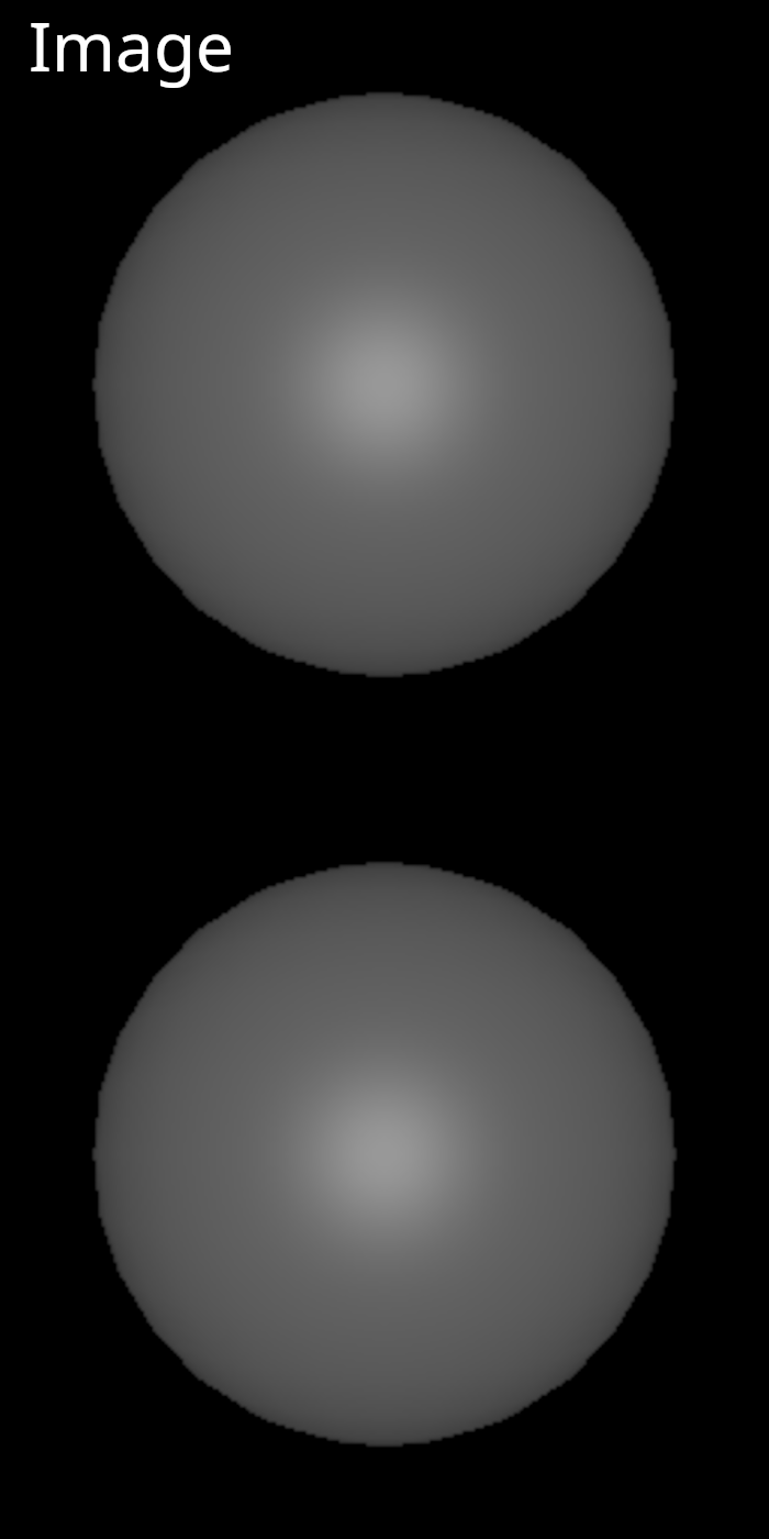
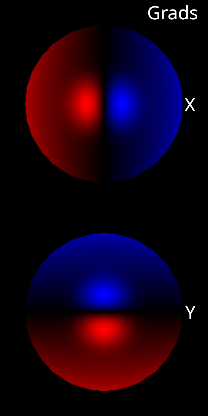
Below, you can see an example image of a Blinn-Phong shaded sphere illuminated by a single, white directional light facing the same direction as the camera. You can also see two different Jacobian images that correspond to the \(x\) and \(y\) components of the light direction parameter. The Jacobian images correctly show how the brighness of the sphere will change when the light is tilted up/down or left/right. They capture both the specular and diffuse aspects of the shader.
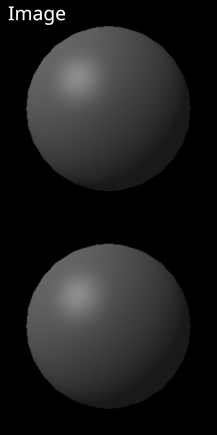
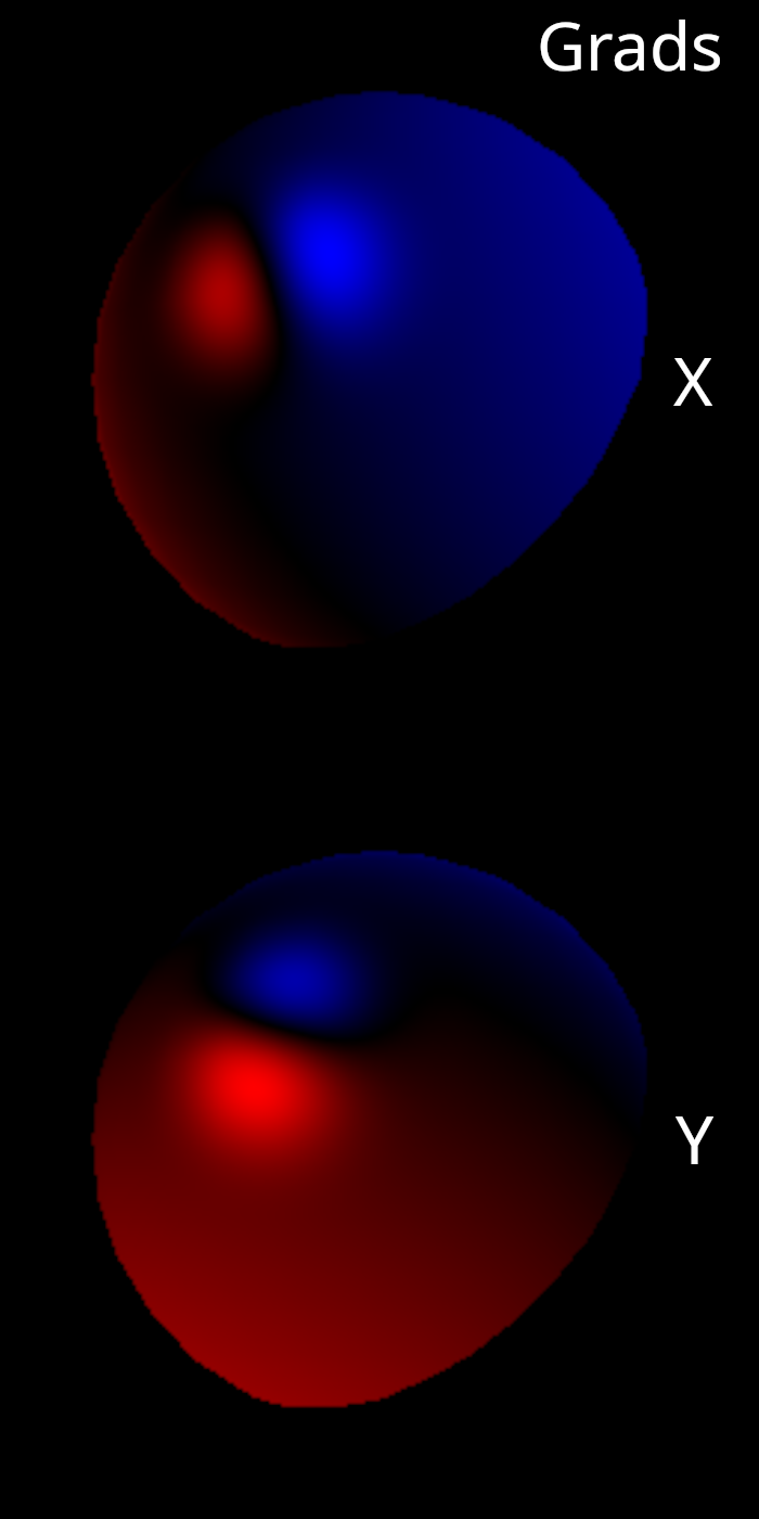
Below, we have repeated the same experiment with a slightly different initial light configuration. Again, the gradient images correctly show how the brighness of the sphere will change when the light is tilted up/down or left/right. We can also see that the derivative is zero at pixels where the diffuse and specular shading contribution is zero.
These gradient images are a very helpful and intuitive way of checking that our gradient computation is functioning properly. Let’s also take a moment to appreciate that we were able to compute these gradients without writing a single extra line of code to implement a VJP. Taichi took our shading kernel and compiled a VJP function all on it’s own. We can now edit our shading kernel (so long as we obey the AD rules) and the VJP kernels will be automatically updated to stay in sync with a new shading approach. If it wasn’t already clear to you, hopefully you can now see why AD is such a powerful technology!
It’s also worth noting that we have obtained gradients for our light parameters without having solved the discontinuity problem! Only the rasterization step in our pipeline is affected by this problem and the shading and light parameters only appear after the rasterization buffers. Therefore we will be able to perform inverse rendering perfectly well for this part of our pipeline.
Coding Challenge 5
The coding challenge for this lesson is to implement your own version of the experiments described above. This mostly involves making use of the existing rendering pipeline combined with the AD functionality of Taichi. As always, we will provide some additional discussion about our implementation below. You can also go look at the project codebase to see exactly how our implementation works.
Implementation
We will start with the same rendering pipeline that we developed in the last lesson.
@ti.data_oriented
class Pipeline:

    def __init__(
        self,
        resolution=(1024, 1024),
        mesh_type="dragon",
    ):

        self.camera = tdr.PerspectiveCamera()
        self.mesh = tdr.TriangleMesh.get_example_mesh(mesh_type)

        self.rasterizer = tdr.TriangleRasterizer(
            resolution, self.camera, self.mesh, subpixel_bits=4
        )
        self.world_position_interpolator = tdr.TriangleAttributeInterpolator(
            vertex_attributes=self.mesh.vertices,
            triangle_vertex_ids=self.mesh.triangle_vertex_ids,
            triangle_id_buffer=self.rasterizer.triangle_id_buffer,
            barycentric_buffer=self.rasterizer.barycentric_buffer,
        )

        self.normals_estimator = tdr.NormalsEstimator(mesh=self.mesh)
        self.normals_interpolator = tdr.TriangleAttributeInterpolator(
            vertex_attributes=self.normals_estimator.normals,
            triangle_vertex_ids=self.mesh.triangle_vertex_ids,
            triangle_id_buffer=self.rasterizer.triangle_id_buffer,
            barycentric_buffer=self.rasterizer.barycentric_buffer,
            normalize=True,
        )

        self.vertex_albedos = ti.Vector.field(
            n=3, dtype=float, shape=(self.mesh.n_vertices), needs_grad=True
        )
        self.albedo_interpolator = tdr.TriangleAttributeInterpolator(
            vertex_attributes=self.vertex_albedos,
            triangle_vertex_ids=self.mesh.triangle_vertex_ids,
            triangle_id_buffer=self.rasterizer.triangle_id_buffer,
            barycentric_buffer=self.rasterizer.barycentric_buffer,
        )

        self.light_array = tdr.DirectionalLightArray(n_lights=1)
        self.light_array.set_light_color(0, tm.vec3([1, 1, 1]))
        self.light_array.set_light_direction(0, tm.vec3([1, -1, -1]))

        self.phong_shader = tdr.BlinnPhongShader(
            camera=self.camera,
            directional_light_array=self.light_array,
            triangle_id_buffer=self.rasterizer.triangle_id_buffer,
            world_position_buffer=self.world_position_interpolator.attribute_buffer,
            normals_buffer=self.normals_interpolator.attribute_buffer,
            albedo_buffer=self.albedo_shader.output_buffer,
            ambient_constant=0.1,
            specular_constant=0.2,
            diffuse_constant=0.3,
            shine_coefficient=30,
        )

        self.output_buffer = self.phong_shader.output_buffer

    def forward(self):
        self.camera.forward()
        self.rasterizer.forward()
        self.world_position_interpolator.forward()
        self.normals_estimator.forward()
        self.normals_interpolator.forward()
        self.albedo_shader.forward()
        self.phong_shader.forward()
For these new experiments we also need a backward method for our pipeline and for our shader. Thanks to the AD functionality of Taichi, this is extremely easy.
# Pipeline
def backward(self):
    self.phong_shader.backward()

# Blinn-Phong shader
def backward(self):
    self.shade.grad()
Now we wish to compute some Jacobian images using reverse-mode AD. We start by creating a couple of arrays to hold our Jacobian images. Next, we populate each pixel in the image. To do this, we run forward on our pipeline, we seed the gradient at the pixel of interest, and we backpropagate the gradients to our light parameter fields. Finally, we grab the value of interest from the gradient field and copy it into our image buffer. Pretty simple!
x_grad_image = np.zeros(shape=(x_resolution, y_resolution))
y_grad_image = np.zeros(shape=(x_resolution, y_resolution))

for x in range(x_resolution):
    for y in range(y_resolution):
        pipeline.forward()
        pipeline.output_buffer.grad[x, y, 0] = tm.vec3([1.0, 1.0, 1.0])
        pipeline.backward()

        x_grad_image[x, y] = pipeline.light_array.light_directions.grad[0].x
        y_grad_image[x, y] = pipeline.light_array.light_directions.grad[0].y
Conclusion
In this lesson we did a deep dive into AD and talked about Jacobians, vector Jacobian products, and Jacobian vector products. We learned how to generate Jacobian images that are very helpful for evaluating whether AD is working properly. In the next lesson we will perform our first real piece of inverse rendering!